Music and machine learning - Group A
Performing with the Wekinator
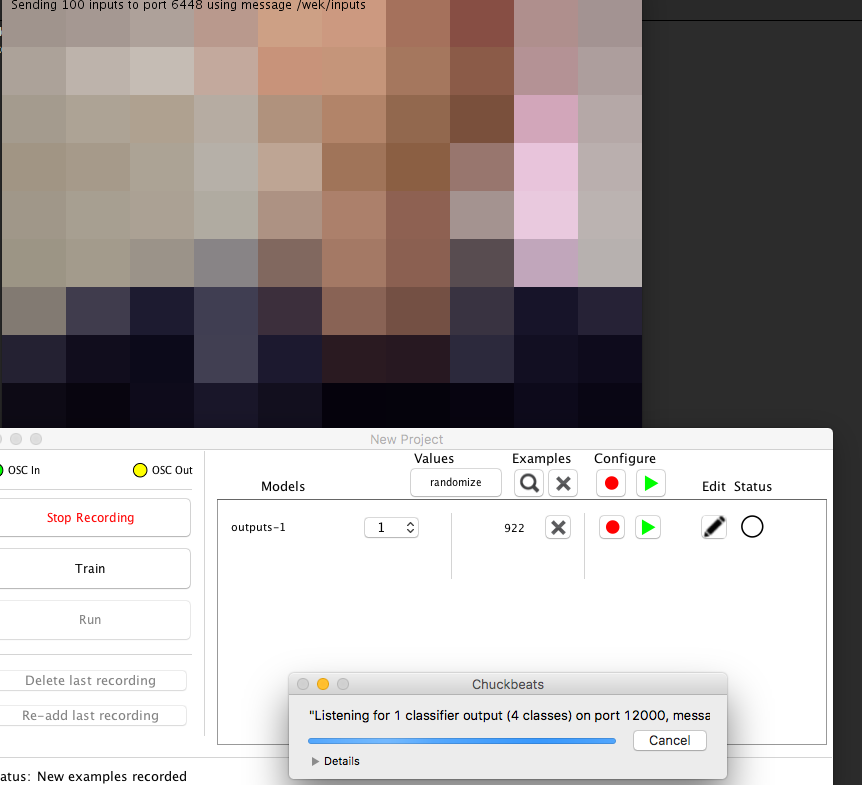
We started out with choosing an input method, and later discussed how to make the algorithm learn behaviour from the input and transform it into meaningful audio. The final system consisted of a web camera feed as its input (100 averaged pixel values) and drum machine patterns as targets. The Wekinator was used to classify colors from the web camera feed, and map those color classes to trigger pre-determined patterns in the drum machine, i.e. “blue” corresponds to pattern A and “red” corresponds to pattern B. In total there were four patterns to trigger in the drum machine, which suggested choosing four as the number of classes for the classification algorithm.
Part of our plan was to send the web camera from Oslo to Trondheim, and then to train a model in Trondheim. Although we initially managed to set up an OSC stream over UiO’s VPN over the UDP protocol, something with the routing failed on the presentation day. The presentation of the model was therefore done locally, but with the same ML principles.
Due to the development context of the system, there were certain aspects of the system that were easier to deal with than it would be in a real world application. The problem of overfitting did not apply in this context, because the model would only be used for a one-time scenario. Another implication of the context was that the amount of training data needed was fairly small. After several rounds of testing, the conclusion was that only around half a minute of web camera recording (800 frames of 30 FPS) in total were needed to train a rough classifier on four different color states. Most of these seconds were used to record the background, to establish a stable base class for the classifier. If the system were to be regularized and made production ready, e.g. as a DAW plugin, a lot more effort would have had to be put into training the model with different kinds of data. Inferring the model with new data from a separate testing and validating set would be a high priority before deploying such a system in production.
Classifying sounds with scikit-learn
We explored the Python library scikit-learn to learn more about how machine learning algorithms can be used for classification of different sounds.
Audio Data Classifier
Divided into three groups, each team got the task to classify a set of 200 audio files in four distinct classes. To implement the data classification, we used scikit-learn library. Each of the four classes was equally divided into 50 files, previously defined by the team members based on audio features that could be distinguished by humans, not requiring special expertise in audio analysis.
Our group selected the following classes: modular synths, orchestral, nature environment, and birds. We had to classify the dataset that we created, and also, the dataset provided by the group B, with the classes glass, stone, wood, metal.
Methods
In the beginning of this process, we had a shallow acknowledgment on how the parameters would affect the machine learning performance, so the first step was to make individual changes for each parameter that we had a previous understanding on the correlation with relevant audio features for the task.
Starting the tests with the Group A dataset, we chose key parameters such as sample rate, and the number of max iterations, making notes on how each setting affected the performance of the classifier. After that, we gradually increased the complexity of the parameters changed, diving into a deeper interaction with the machine learning process. Thus, we started to adjust parameters such as activation, hidden_layer_sizes, and extract feature’s.
One important decision was to always try to use the minimum computing process power reasonable for the maximum accuracy goal, meaning that for each parameter tweaked, we considered only meaningful changes, avoiding overfeeding the model with irrelevant audio information, and consequently, confusions in the learning process.
In this way, it was noticeable that for the dataset A, increasing the sample rate to 24kHz, improved the accuracy of the results, since some audio sets, such as birds, for example, have relevant frequency information relying above 10kHz. Next, we started to interact with the machine demands. From changing the activation parameter, we could observe how effective was to increase or decrease the max_iter values. The tanh activation combined with max_iter=3300, worked well to the demand, and when increased the iterations to values above 3500, the results got less precise.
Arranging the neural network, we observed that the results improved when increased the number of layers and neurons from hidden_layer_sizes=(2,2) to (6,8,4), but more than that did not give me better results. After enlarging the size of the network, consequently, the machine required more iterations, becoming max_iter=8800 an optimal value.
At this stage of the process, after testing different features in parallel with the previous settings, we realized the best combination of features that fit better for each dataset.
We used the same method to achieve satisfactory results with the dataset B, but with a bit more experience with the parameters, we could use a more objective approach.
Results / Discussion
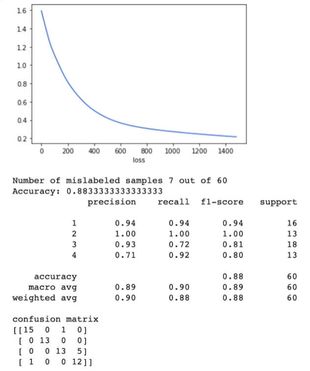
In the case of the dataset A, the best feature arrangement was spectral_centroid and spectral_bandwidth, delivering better results than the default setting (zero_crossing_rate). It is probably due to the distinct spectral characteristics of the classes, having different located mass of energy in the spectrum.
As you can see in the graph below, the worst precision result came from class 4 (Birds). Probably due to the inconsistency among the duration of the audio files of this set, in addition to the background noise captured in the recordings.
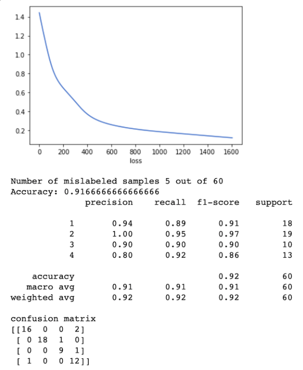
For the dataset B, the sample rate optimal value had to be much higher to deliver better results, ending up with 44.1kHz. The activation and the neural network were very similar to the ones selected to the dataset A, but the max_iter of 5500 fit better, delivering worse results if increased.
However, the feature extraction required to dataset B was way different. The best combination of features was spectral_ bandwidth with spectral_ flatness. It makes sense, considering that spectral flatness is a tonality coefficient and combined with the spectral bandwidth, they can be very effective to distinguish sounds that have peculiar and clearly distinct tonal characteristics such as glass, stone, wood, and metal.
With dataset B, we got the best accuracy results, relying around 92% as you can see in the graph below. Also, the worst precision came from class 04 (Metal). Probably because the spectral bandwidth variety among the audio samples was large, being hard to identify a standard pattern regarding the wavelength.