Sonifying the Northern Lights: Two Approaches in Python & Pure Data

Introduction
The weekend of 31 October 2003 passed like any other Halloween, unless you happened to be in Spain or Texas. If you did, you would have seen something you might have never seen in person before: the Aurora Borealis. Halloween 2003 is the period of highest intensity of solar winds, which cause the Northern Lights, since modern records began. Your three authors have spent two weeks deeply immersed in the solar winds data from the week of Halloween 2003, which saw possibly the biggest solar event since 1859.
Our final two group assignments for MCT4001 were to sonify a dataset using both Python and Pure Data. Here is a deep dive into how and why we sonified this data in the ways we did.
About Our Dataset
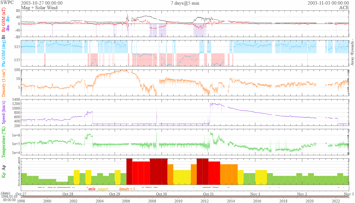
We pulled our data from the Space Weather Prediction Center’s online dataset which has data going back to 1998. The SPCC, which is operated by the US National Oceanic and Atmospheric Administration, collects solar wind data from two different measuring satellites positioned around 1,500,000 miles / 2,400,000 km forward of Earth, as well as various Earth-based measurements. Their website allows us to get readings from every minute for the last 24 years, so we pulled the data from the period of 27 October - 2 November 2003, a period of 7 days, and then performed data cleaning that includes removing erroneous measurements and interpolating to fill the gaps. Finally, we computed 5-minute averages, which resulted in 2016 individual readings across the period. Each reading contains 10 different data points, of which we used 7 in each sonification.
The data we used is shown in the table below:
| Data Type | Data Point | Units | Measured from | What does it mean? |
|---|---|---|---|---|
| Physical | Proton density | /cm3 | ACE satellite | The density of the protons in the ionised gas that makes up the solar winds. |
| Ion Temperature | Kelvin | ACE satellite | The temperature of the ions in the solar winds. | |
| Bulk speed | km/s | ACE satellite | The speed of the solar winds. | |
| Magnetic | Bz | nanoTeslas | ACE satellite | The strength of magnetic field of the solar winds (called the interplanetary magnetic field or IMF) in the z-axis i.e. North/South. |
| Bt | nanoTeslas | ACE satellite | The overall strength of the IMF. | |
| Phi angle | Degrees | ACE satellite | The resulting angle from the horizontal Bx and By components of the IMF’s magnetic field. | |
| Synthetic | Kp-index | No units (0-9) | Earth | A weighted average of the K-index at 13 different locations around the planet. Measures the disturbance in the horizontal component of Earth’s magnetic field. |
Sonifying in Python
For our assignment we were required to use a corpus of pre-recorded music to sonify our dataset in Python. We eventually settled on using the song at number one in the charts in Norway over the Halloween weekend 2003; Dido’s White Flag. Inspired by the cloud of ionised gas that makes up the solar winds, we decided to sonify the data using clouds of sound with granular synthesis.
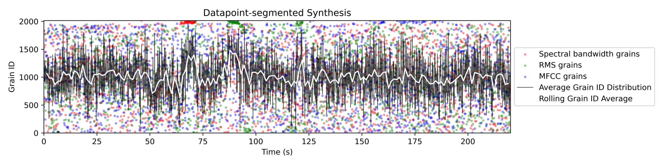
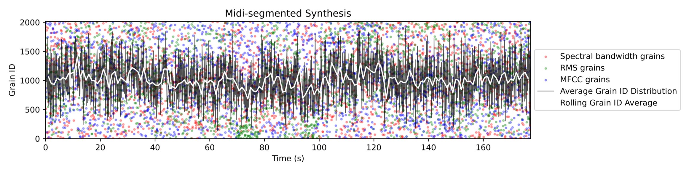
We divided the song into ‘grains’ in two ways: by dividing the song equally by the length of the dataset (we call these the data point grains), and by using a MIDI representation of the song to split it into pieces each one 32nd note in length and quantized to the beat (we call these the MIDI grains). The first method resulted in grains around 109 ms in length, while the second resulted in grains around 88 ms in length.
Mapping with Feature Extraction
Mapping data to musical processes and parameters is an essential part of any sonification, and we mapped in two distinct ways. Firstly, we developed rules based on the individual data points for choosing what grains should be played at any point in the sonification. Secondly, we mapped the remaining data points to different audio effects and transformations.
To map individual grains to individual data points, we performed three types of feature extraction on each grain using the Librosa library in Python:
- Spectral bandwidth, which measures the deviation from centre of mass of a signal and is an indicator of the timbre of a sound
- Mel-frequency cepstrum, which provides coefficients for the power of a sound in different frequency bands. From these coefficients we took the largest coefficient value.
- RMS, which measures the average power of a signal
Each of these features resulted in a single number value per feature per grain. We used these numbers to rank the grains by each of their features. We also ranked our dataset by proton density, ion temperature, and Bz values. We then matched lowest to lowest between grains and values in the dataset, such that the grain with the smallest value in a certain feature corresponds to the smallest value in a particular datapoint. This mapping went as follows:
- Proton density mapped to spectral bandwidth
- Ion temperature mapped mel-frequency cepstrum
- Bt values mapped to RMS
This resulted in each of the 2016 readings in our dataset corresponding to 3 different grains from the song, one for each feature-reading mapping.
Mapping with Audio Processing
Having now decided which fragments of our audio corresponded to which readings in the dataset, we mapped the rest of our variables using different types of audio processing:
Bulk speed determined the playback speed of each grain, within a range from half to double the original speed Phi angle determined the playback direction, such that if the value was below a threshold, the grain played in reverse Bz mapped to the type and cutoff frequency of a filter. A low-pass filter was used for values above 0 and a high-pass filter for values below 0, while the absolute value of the reading was scaled as the cutoff Kp-index mapped to the dry/wet parameter of a convolution reverb
Building the Sonification
Having now mapped every value in our data to a grain or audio processing parameter, we assembled our sonification by moving through our dataset in chronological order. We pulled the three corresponding grains for each reading, layered them on top of each other, and then applied the processing to this summed grain. We repeated this process for both of the grain types. You can listen to the results below:
Reflections
After hearing the result of our Python sonification, we decided to produce a scatter plot for each grain type to show which grains were mapped to which points in the data. We expected grains that were close to each other in the original song to provide similar values from feature extraction, and therefore that we would see some clustering when these were mapped to the data. There were a few instances of clustering, but far fewer than we expected. Plotting the average grain ID for each reading in the dataset, we see that while there is some deviation, the average grain ID is quite normally distributed.
As seen in the figures below, our segmentation approaches resulted in slightly different selection of grains. However, neither shows any strong relationship between the location in the dataset and location in the original song from which the corresponding grains are taken.
We also produced a dynamic visualisation of our dataset time-synced to the audio produced by both grain types. You can see the results of this for the data point grains below:
Sonifying in Pure Data
Sonification in Pure Data was an entirely different challenge to doing it in Python. Pure Data is built as a real-time, often interactive audio and music programming language. Unlike Python, where we can use the Pandas library to conveniently handle large datasets in an Excel-like format, Pure Data forced us to handle our data in a different way.
Accessing Our Dataset in Pure Data
We found the easiest way to store a dataset in Pure Data was in arrays. Arrays in Pure Data work much like lists in a coding-based programming language like Python. We provide a specific index, or position in the list, and get back the value stored there. For example, if we provide the number three, we will get back the third value stored in that array. Attaching this behaviour to a metronome which increments by 1 at regular intervals, we can move through our data in chronological order at a tempo we set. We then use the values we get back to affect parameters of other things we make in Pure Data like synthesisers or audio effects.
This logic forms the basis of our sonification in Pure Data. We exported each of our 7 data points into text files, and then loaded those into Pure Data arrays. A ticking counter then requests the value from the same position in each of the arrays. We then have the 7 values for a particular reading in the dataset, which we can scale and transform to adjust a vast number of parameters in the Pure Data patch.
Mapping
In Python we used a pre-existing song as the basis for our sonification. However in Pure Data we sonified the dataset from scratch using a variety of drum machines, sequencers, synthesisers, audio effects and other modules that we built during the semester.
We use our data to control the resulting music in two different ways:
- Direct mappings - there is a one-to-one relationship between data and parameter. For example, density is mapped to the pitch of the lead and bass synths. If the value in the data increases, the parameter increases. This relationship is sometimes inverted, but the mapping is still considered direct.
- Generative mappings - the data controls the behaviour of other algorithms which in turn control parameters. For example, the bulk speed data controls the amount of hits in the kick drum pattern. The data does not specify specifically when the kick should be triggered, only the frequency with which it should be triggered.
The full table of our mappings is below:
| Data Point | Mapped To | Mapping Type | Notes |
|---|---|---|---|
| Proton density | Lead synth pitch | Direct | Sometimes quantized to MIDI notes, based on bulk speed mapping below. Adjustable tempo i.e, the user can change how often a reading from the dataset generates a note. |
| Bass synth pitch | Direct | Quantized to MIDI notes. Adjustable tempo i.e, the user can change how often a reading from the dataset generates a note. Inverted from lead synth pitches. | |
| Lead synth note probability | Generative | The chance that the lead synth plays a note when it receives a new frequency. | |
| Ion temperature | Lead synth spread parameter | Direct | Spread is the degree of variation in pitch between the different oscillators in each synth voice. |
| Snare pattern density | Generative | Changes the probability of triggers in the snare pattern, therefore controlling the density of the pattern. | |
| Bulk speed | Lead synth chorus effect parameters | Direct | Affects all three parameters of the first chorus effect equally. |
| Lead synth midi quantization | Direct | Tells the synth to use MIDI quantized frequencies below a certain threshold, and use the raw unquantized value above the threshold. | |
| Kick pattern density | Generative | Changes the probability of triggers in the kick pattern, therefore controlling the density of the pattern. | |
| LFO speed | Direct | The LFO in turn modulates several parameters of the bass synth and its effects. | |
| Bz | Lead synth chorus effect parameters | Direct | Affects all three parameters of the second chorus effect equally. |
| Bt | Lead synth filter cutoff frequency | Direct | Affects the peak of the filter envelope. |
| Closed high hat pattern density | Generative | Changes the probability of triggers in the closed high hat pattern, therefore controlling the density of the pattern. | |
| Phi angle | Lead synth delay parameters | Direct | Affects the delay time, dry/wet, stereo effect and feedback level. |
| Lead synth envelope attack & release | Direct | Values below 225 set attack time in ms, values above 225 set release time in ms. | |
| Bass synth envelope attack & release | Direct | Values below 225 set attack time in ms, values above 225 set release time in ms. | |
| Open high hat pattern density | Generative | Changes the probability of triggers in the open high hat pattern, therefore controlling the density of the pattern. | |
| Kp-index | Bass synth reverb amount | Direct | Controls the dry/wet parameter. |
Building the Sonification
Once our mappings were set, the process of sonifying our data was as simple as pressing play on the counter and letting it run. However, we also added some extra some extra functionality to our counter to allow the user to set variable start and end points, toggle looping and going in reverse through the dataset, and increment and decrement in individual steps for finding precise points in the data. As the control mechanism is essentially a metronome, we can also change the tempo and the subdivisions of the beat for each of the lead, bass and drum lines. The user can also change some parameters during the sonification, such as locking the drum patterns for a period of time, which can help to ‘tame the beast’ that is our patch.
We added a simple recording module to the end of the patch to write the output to a file, and with that, our Pure Data sonification was complete.
You can listen to the entire thing here:
Or watch a shorter video showing part of it here:
Reflections
Because the sounds used in our Pure Data sonification are built from scratch rather than sampled from a pre-existing song, the relationship between the data is generally more noticeable to us than in our Python sonification. However, we are now very familiar with the shape of our data. To a casual listener, the shape of the data is likely not identifiable apart from at a few key moments when the data changes rapidly and therefore so does the sonification.
We are generally happy with the result of our Pure Data patch. The sound is very chaotic, but this is to be expected when almost every parameter beside tempo is constantly changing. When combined with several user controls to lock the drum patterns and affect synth behaviour, the result is quite performable.
Downloads & Links
- GitHub repo for our Python sonification here.
- White Flag by Dido.
- We downloaded our dataset from Space Weather Prediction Center here.