MCT Blog Sonified!

This blog has been held by students and alumni of the MCT program for the last four years. Today, it contains 370+ posts about topics ranging from audio programming to musical interaction, concerts, and experiences. According to wordstotime.com, to read this beautiful blog entirely, you would spend 286 hours. But don’t worry, you can listen to it!
Before we dive into this, here are some fun facts about our blog!
- Amongst 2334573 words typed in the blog so far, the three most frequent words were audio, sound, and music.
- The word We was used 1.43 times more than the word I.
- The longest word in the MCT blog is multiinstrumentalist with 20 characters - if we don’t count the word reverberaaatioooooooon with 22 :)
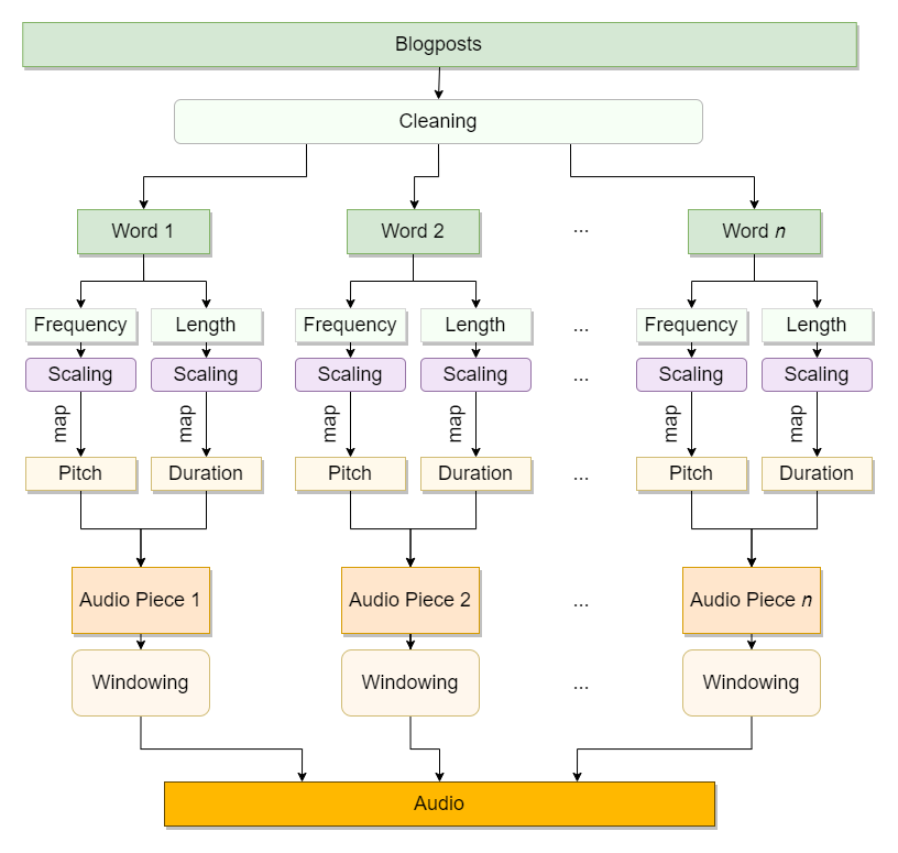
To make a sound out of data, it should be in the shape we want it to be. Cleaning, arranging, and scaling are crucial, especially in appropriately mapping the data to specific parameters. Then, we can create sound based on the numbers at hand. For this data, I started off by excluding some parts of the texts, removing unwanted words and filtering. Then, I scaled it before mapping it to specific sound parameters. Finally, these numbers turned into sound. Diagram below shows this sonification process.

Gathering the Data
The MCT Blog runs on GitHub Pages with a GitHub repo in the background, which allowed me to get each blog as a seperate file in markdown format. Each post had the same structure: a frontmatter with meta information (e.g., date, tags, authors), blog post content in markdown format with links to images, videos, and embedded elements. This structure made the data cleaning relatively more manageable.
I started cleaning the data by excluding the frontmatter from each file, which basically contains repetitive out-of-context words. Next, I scraped out markdown signs using BeautifulSoup. I cleaned the data further using a set of regular expressions, including lowercasing, removing punctuations, and cleaning white spaces.
path = './_posts'
files = os.listdir(path)

# iterate files, remove frontmatter and parse to get text
all = ''
for i, file in enumerate([s for s in files if s.endswith('.md')]):
    text = ''
    with open(os.path.join(path, file), encoding = 'utf-8') as f:
        md = f.read()
        md = re.sub("\n", " ", md)
        md = re.sub(r"---.*---", '', md)
        html = markdown.markdown(md)
        soup = BeautifulSoup(html, features='html.parser')
        text = soup.get_text()
        all += text

# clean text
cleaned = all.lower()
cleaned = re.sub("(\[.*\])", "", cleaned)
cleaned = re.sub("(http[s]?\://\S+)", "", cleaned)
cleaned = re.sub("[0-9]", "", cleaned)
cleaned = re.sub("\S*@\S*\s?", "", cleaned)
cleaned = re.sub("/\S+/\S+", "", cleaned)
cleaned = re.sub("\n", " ", cleaned)
cleaned = re.sub(r"[^\w\s]", "", cleaned)
cleaned = cleaned.translate(str.maketrans('', '', string.punctuation))
cleaned = re.sub("\s+", " ", cleaned)

# save all words
with open('all_words.txt', 'w', encoding='utf-8') as f:
    f.write(cleaned)

words = cleaned.split(' ')
df_words = pd.DataFrame(words, columns = ['words'])
The steps above resulted in having an array of cleaned words. Next, I cleaned the outliers, words such as “all”, “and”, “to”, words that are too long, and words that are too much or less frequent.
# remove unwanted words, remove extremes
unwanted_words = ['', 'the', 'to', 'and', 'of', 'a', 'in', 'is', 'for', 'with', 'that']
df_words = df_words[~df_words['words'].isin(unwanted_words)]
df_words['w_len'] = df_words['words'].str.len()
df_words = df_words[(df_words['w_len'] > 1) & (df_words['w_len'] < 20)]

# calculate frequencies, remove less frequent
counts = Counter(df_words['words'])
df_freq = pd.DataFrame(counts.most_common(), columns=['words','freq'])
df_freq = df_freq[(df_freq['freq'] > 10) & (df_freq['freq'] < 1500)]

df = df_words.merge(df_freq, how='left')
df = df.dropna()
Data Preprocessing and Mapping
After the first cleaning part, words’ frequency of appearing in the entire blog gave me values ranging from 11 to 1323. I simply scaled it up by 10. The word lengths ranged from 1 to 15. I multiplied it by 2, to use as length (ms) of each audio piece. Also, this can be scaled globally in the final step using the speed variable.
# scaling
df['freq'] = df['freq']*10-90
df['w_len'] = df['w_len']*5
Sonification
For every word, I generated short audio samples, which come together to create a musical piece. I decided to map each word’s frequency (i.e., how many times each appeared on the website) to the leading pitch. I used each word’s length as the duration of each audio sample. This way, I expected to obtain a sound pattern that reflects the characteristics of the text (i.e., more frequent words sound high-pitched, and longer words make longer sound).
I ended up having 5.6 ms long audio pieces generated for each word on average. I applied hamming window to each, and combined them one after another, to have a piece of music! Code below does the job.
# sonify

sr = 48000
sr_ms = int(sr/1000)
signal = np.array([])
l = len(df.index)
speed = 0.5
for i, row in df[:2000].iterrows():
    freq = row['freq']
    note_dur = row['w_len']/speed #ms
    start_sample = i*note_dur*sr_ms
    dur_sample = note_dur*sr_ms

    # sin wave
    f = freq
    A = 1
    t = np.arange(0,note_dur/1000,1/sr)
    s = A*np.sin(2*np.pi*f*t)

    # window
    window = scipy.signal.windows.general_hamming(len(s), alpha=0.5)

    # append
    signal = np.concatenate((signal, s*window))

sf.write('mct_blog_sonified.wav', signal, sr)
