Creating Complex Filters in Pure Data with Biquad~

An Brief Introduction to Filters

Coffee filters and audio filters work on much the same principle. A coffee filter lets your lovely hot coffee through while preventing bits of bean from ending up in your oat milk flat white. Meanwhile digital filters let through some frequencies (the coffee) while holding back others (the coffee grounds). Audio filters are one of the key components of the computer musician’s toolbox. As musicians, we most commonly think of filtering as a component of mixing or sound design. However, a filter can be applied to any time series data, for example control signals in Max/MSP or Pure Data, physical sensor data, or even geological data or tidal data.

The most used filter types in musical contexts are low-pass, high-pass, band-pass, and band-stop, which work largely as the names suggest. However, one can also specify more complex filter shapes. For example, suppose we want to correct or ‘flatten’ the natural frequency response of a room or a pair of headphones. A simple low-pass filter is not going to be enough, as there are numerous frequencies that are either boosted or attenuated to different extents. As a result, we will need to employ a filter with a complex response to neutralise the peaks and valleys.

An example of a complex filter response in Sonarworks software, which aims to flatten the frequency response of my headphones.

Designing Complex Filters in Python & Pure Data

Designing a complex filter in Python is made relatively straightforward using the Signal component in the SciPy library. We simply call an appropriate function, specify our requirements, and the rest is taken care of under the hood. Meanwhile, the Pure Data graphical programming language offers some user-friendly objects for the common filter types mentioned above as well as some more daunting algorithms. However, it does not have a one-stop solution for building complex filters of the sort we can specify in Python. Instead we can ‘cascade’ several simpler filter shapes together to recreate a more complex response. For example, we can use low-pass and high-pass filters together to create a sufficient, if fairly imprecise, band-pass filter. For more precise filter requirements in Pure Data however, we can turn again to SciPy.

Recreating a Python Filter in Pure Data

SciPy’s handy tf2sos() function allows us to break down an IIR filter designed in Python using a function such as into a series of simpler sections. Each of these second order sections, of which there can be many, can then be interpreted by a biquad~ filter in Pure Data to recreate our complex filter.

The tf2sos() function returns a list of lists of filter coefficients that define the frequency response of each section. Below is one approach to recreating in Pure data an IIR filter built with SciPy. It uses Python to run a terminal command which opens Pure Data and sends lists of filter coefficients to Pure Data receive objects. These lists which are the interpreted by multiple biquad filters to recreate the original complex filter. This approach allows for filters of IIR filters up to order 16 to be accurately recreated in Pure Data. A small amount of precision is lost in translation due to the difference in accuracy of floating point numbers between Python and Pure Data. However this is negligible for our audio examples below.

In Python I piece together a terminal command to open the Pure Data patch and pass the filter coefficients as lists using the -send command line option. This option allows me to send directly to ‘receive’ objects in Pure Data by simply providing the name of the receive and the data I want to send to it. In this case, lists of numbers are passed via receive objects to several biquad~ objects to recreate the filter, and the resulting sound is written to the specified audio file.

The Python code builds the following command:

C:/Program Files/Pd/bin/pd.exe -open tf2sos_biquad.pd -r 48000 -send "; sec1
0.7259912605703875 -0.0 0.03806324928680216 0.03806324928680211 0.0; sec2
1.7126604844375657 -0.7597960137277255 1.0 -1.8856873367725067 0.9999999999999819;
sec3 1.9117563444113768 -0.9417048830803751 1.0 -1.9555513841911991
1.000000000000015; input_file ./test_audio/to_be_filtered.wav; output_file
./test_audio/filtered_pd.wav"

The code that builds this command is:

def __pd_build_command(sos_scaled, input_file, output_file):
    """Builds the command given the Numpy array of coefficients and
    the input and output filenames."""
    
    # Pd install directory
    pd_executable = "C:/Program Files/Pd/bin/pd.exe"
    pd_patch = "tf2sos_biquad.pd" # The Pd patch to open
    
    # Initialises empty list which will contains strings of coefficients
    section_strings = []

    # Initialises string containing all sends
    sends = ' -send "' 

    coeff_order = [4,5,0,1,2] # List of new order for coefficients

    # Loops through the second order sections, which are all stored in a Numpy array
    for sec_i, section in enumerate(sos_scaled):
        coeff_string = "" # Initialising/resetting the string of coefficients
        for i in coeff_order: # iterates through section in required order
            # Appends together the coefficients into a string
            coeff_string = coeff_string + str(section[i]) + " "
        
        # Appends together Pd message for each section
        section_string = "; sec" + str(sec_i + 1) + " " + coeff_string[:-1] 

        sends = sends + section_string # Builds up sends string from section_string

    # Finishes sends string by adding input and output filenames
    sends = sends + "; input_file " + input_file + "; output_file " + output_file + '"'

    # Assembles the final command
    command = pd_executable + " -open " + pd_patch + " -r " + str(sr) + sends

The command first opens the relevant Pure Data patch, sets the sample rate of the patch (48000, the same as I am working with in Python), and then sends lists of coefficients grouped into their sections. These are each received by their equivalent receive objects in Pure Data – the first section is received in ‘receive sec1’ in Pure Data, and so on. Lastly, I pass the path to the file to be filtered and where to save the filtered result. I can also add -batch -nogui to the command, which allows Pure Data to run offline i.e., not in real time and without opening the interface.

While this example only recreates a low-pass filter, this can be theoretically be replicated with any shape of IIR filter designed in SciPy Signal.

The Pure Data patch which receives filter coefficients, filters the audio, and writes the output to a file.

One useful feature of this implementation is its ability to handle IIR filters of various different orders up to 16, which in most cases is a reasonable upper limit for IIR filter order. I included eight second order biquad filters in the Pure Data patch as a 16th order IIR filter was the highest I have encountered so far in Python. However, the tf2sos() function can decompose IIR filters of any order and likewise my Python function which builds the command can similarly handle any number of second order sections. The limiting factor here is the Pure Data patch, although this can be easily expanded to handle larger numbers of sections.

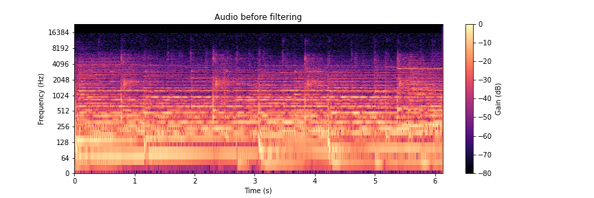
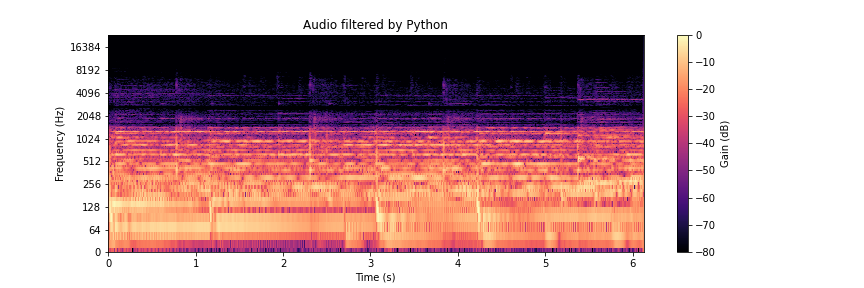
The audio files and spectrograms below demonstrate how both filtering methods produce perceptually identical results.

Audio before filtering

The audio sample before filtering.

Audio filtered in Python using SciPy Signal

The audio sample filtered using SciPy Signal.

Audio filtered in Pure Data using several biquad~ filter in cascade

The audio sample filtered by the same filter recreated in Pure Data.

Downloads

Download the Jupyter Notebook, Pure Data patch, and audio files discussed above from GitHub here.