Chorale Rearranger: Chopping Up Bach
Introduction
It’s interesting to think about the ways in which we store musical information digitally. Different media all provide different levels of access to different precepts of a piece of music. A PDF of the score provides us with information laid out in a logical manner in case we would like to perform it ourselves; however it’s difficult to obtain information about the overall structure at a cursory glance. In comparison, a waveform of a recording of the piece allows us to quickly see the overall structure of the piece’s dynamics, but good luck trying to perform it yourself with only the waveform to work with!
None of these digital representations provide a complete picture of what is happening in the musical work, in fact we might actually receive quite a different impression of a piece depending upon the medium in which it’s presented to us. So what happens if we take the information provided in one medium and start using it to alter the information provided in another? Can we access precepts that are more hidden in one of the types of media? And can we change it to make something completely new?These are the questions that fuelled the development of the chorale rearranger.
If you want to access our Python and Pure Data code it can be found here.
I Hear Voices
Bach’s chorales are settings of Lutheran hymns, with polyphonic harmonisations split between Soprano, Alto, Tenor, and Bass (SATB) voices. When listening to a performance, these voices meld together, forming rich and complex harmony. (As an aside, the chorales were also the focus of a quite well-known computational music project, Deep Bach, where an algorithm was trained to compose music using solely the chorales as input data. Check it out here.)
In a digital representation of a chorale in the form of an audio file, information on the individual voices is inaccessible. We are presented with the complex harmonic and rhythmic interplay of the ensemble, but to pull out information on just one of the voices is an extremely difficult task. And we can completely forget about changing it.
However, there is another digital representation where all of the information on the individual voices is freely available: MIDI. MIDI is simply a way of representing music as a series of note objects, with each note having assigned values on when it should start and end, how loud it should be, and what pitch it is. If you feed this information into a synthesiser capable of parsing MIDI, you will have the piece of music played back to you. However, all of the notes aren’t just jumbled together, but rather are split into separate ‘instrument’ objects, based upon what should be playing them too. So by looking at the MIDI data of a chorale, the information on what each of the voices is doing is immediately clear.
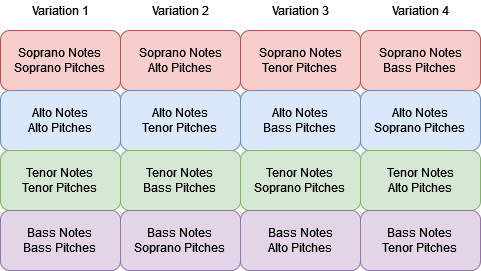
So we came up with a plan: We would take an audio recording and the MIDI representation of one of Bach’s chorales, and based upon the information provided in the MIDI data, attempt to cut into the audio and recreate the individual voices. However, there’s a catch! We would repeat the chorale four times, and in each repetition, we would switch around some of the information in the MIDI data between the voices. Through each repetition we would shift over the pitch of each note by one voice, so that, for example, in the first run through the chorale, the soprano notes would be assigned the soprano pitches, then in the second the alto pitches, then the tenor pitches, then the bass. We hoped that this would reframe the harmonic and rhythmic relationships, and offer a new perspective on the chosen chorale.
Piece and Reconciliation
As we were going to be repeating the chorale four times, we decided to use a relatively short one. We settled upon the 3rd movement from the Matthäus-Passion, which uses the text Herzliebster Jesu, was hast du verbrochen, written by Johann Heermann, set to a melody by Johann Crüger.

We found an audio recording performed by the Collegium Vocale Gent which you can listen to here.
We also found a MIDI file here, which we’ve played back through a synthesiser so that you can listen to it:
The first thing that jumps out is that, even though these are two representations of the same piece, they are actually quite different. They vary in several musical precepts, including tempi, phrasing, and even key! So before we could start cutting into the audio, we had to reconcile these differences.
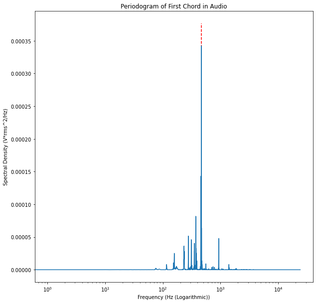
The first precept we attempted to reconcile was the key. What’s interesting here is that we weren’t interested in the objective key of each of the representations, but rather in the respective difference between the two. And because the pitch information for each note is easily accessible in the MIDI data, if we found this difference then we could simply add it to or subtract it from all of this pitch information to put it into the key we want. We also realised that, as this difference in pitch is valid across the whole piece, we didn’t need to find it for the whole, but rather simply for the first chord. So, based upon the start and end times of the first note of the MIDI file, we cut out the first chord from the audio.
As we already had the pitch information of the MIDI data, we now needed to find it for the audio. We realised that if we looked at the audio in the frequency domain, there would be peaks at the fundamentals of the pitches being sung. So we took the periodogram of the audio, calculated the highest peak, then looked at which of the pitches in the MIDI file was closest, calculated the difference, and subtracted it from all of the pitches in the entire MIDI data.
We then re-synthesised the entire MIDI file and layered it on to the audio to check if our method worked. You can listen to this and hear the results yourself!
The next precept that we attempted to reconcile was the tempo. Again, the objective tempi were of no interest but rather the difference. So after applying tempo estimation functions to the audio and the MIDI and calculating the ratio between them, we then multiplied the duration of each note in the MIDI file by it and then once again layered the two to hear if our method was successful.
The final precept, and by far the most difficult, that we attempted to reconcile was the phrasing. If you listen to the audio, you can hear that between the four main phrases of the chorale, the choir takes long, expressive pauses. In contrast, the MIDI file just barrels on through, meaning that the alignment of the notes between the two drifts in and out. If we could also tell the MIDI file to make these pauses, they would theoretically better align.
After trying and failing many times to come up with a method to do this, we settled on taking the amplitude envelope of the audio file and again attempting to find the peaks. However, as we only wanted four peaks, after setting starting parameters, we then iterated over the envelope slowly changing these parameters until only four peaks remained.
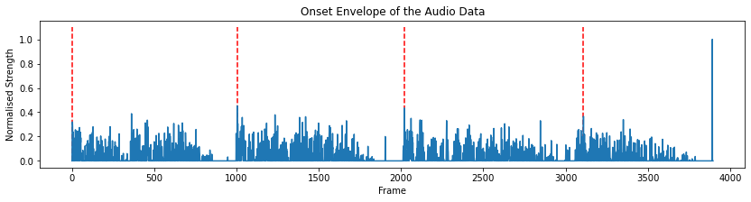
After doing this, we found the MIDI note which had the nearest starting point to the peak, calculated the difference in time between them, and then added or subtracted this difference from all the subsequent MIDI notes’ start and end values. We repeated this step for each peak. Although this method wasn’t entirely successful, you can listen to the layered results below.
With the audio and MIDI reconciled as best we could, we could then start with the rearranging!
Shifting Pitches
The method that we used to chop up the audio for each voice was as follows:
-
Slice the audio between the start and end times of the MIDI note.
-
Apply a narrow band-pass filter to the audio at the pitch of the MIDI note.
-
Pass the audio segment through a saturation function. As the filtering removed a lot of the spectral content, we needed some way to add something back in, and this saturator did the job.
-
Apply a sigmoid window and pad the segment to ensure that there were no clicks when joining the segments back together.

- Append the segment onto the previous segment.

We repeated this process for each of the repetitions, each time shifting the pitch values that we took for the filter by one voice. In addition, with each repetition, we widened the pass band of the band-pass filter to allow more of the original audio through over the course of the piece, hopefully providing the final piece with some more energy over its course.
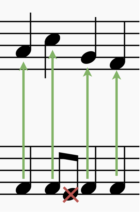
There was a problem however. Each voice doesn’t contain the same number of notes, so when taking the pitches from the notes of one voice and applying them to the segments sliced using the note durations from another we had to decide how to assign them and what to do with the excess values.
Our first idea was to relate the assignment to the timing of the original piece. This would mean that if there were subdivisions in the note duration of one voice in relation to a single note in the voice that the pitches were being taken from, both of these subdivided notes would be assigned the pitch of the single note. This would also be the case in reverse, so that if the voice from which the pitches were being taken had subdivisions, only the pitch from the first of these subdivided notes would be applied to the longer note in the voice in which the pitch was being assigned to.
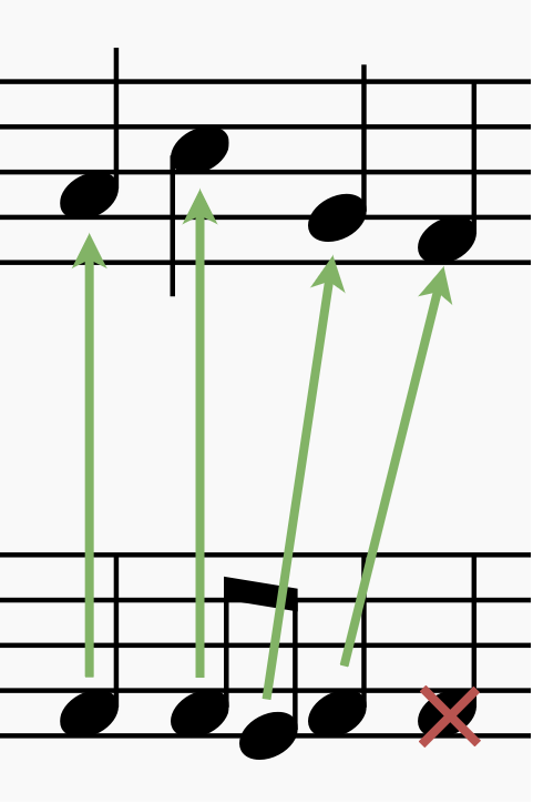
However, we realised that if we did this, there wouldn’t be so much shifting in the harmonic contexts of our final piece. So we came up with another idea.We would just run through each of the pitches in turn, with each note being assigned the following pitch sequentially. If the voice being assigned the pitches had fewer notes than the voice from which the pitches were being taken from, the last of these pitch values would be discarded. In the opposite case, the final notes would just hold on the final pitch.
This resulted in the harmonies shifting for each repetition, sometimes building dissonances and sometimes creating new consonances.You can listen to the result here:
However, this still sounds a little raw. So we decided to apply some processing to make it sound a little more like we imagined.
Trust the Process
The first step we took to process the audio was to underlay it with pure sine tones at a low volume. We did this by using the same steps as we did to process the audio, except instead of using the information provided by the MIDI file to chop the audio, we used it to generate the sine waves. This made the pitches become clearer and the consonances and dissonances easier to follow.
After this, we passed the audio file through to Pure Data to apply some light reverb and parallel filters with shifting centre frequencies to create some subtle movement.
After passing the audio back into Python, we convolved our piece with the impulse response (recorded by Nick Green) of the silo of a Maltese citadel in order to provide an ethereal, open sense of space.
Our final, rearranged chorale sounds like this:
The first variation sounds similar to the original, but as the variations continue, the textural consonances and dissonances start shifting, recontextualising what we just heard. We were pretty happy with the results!
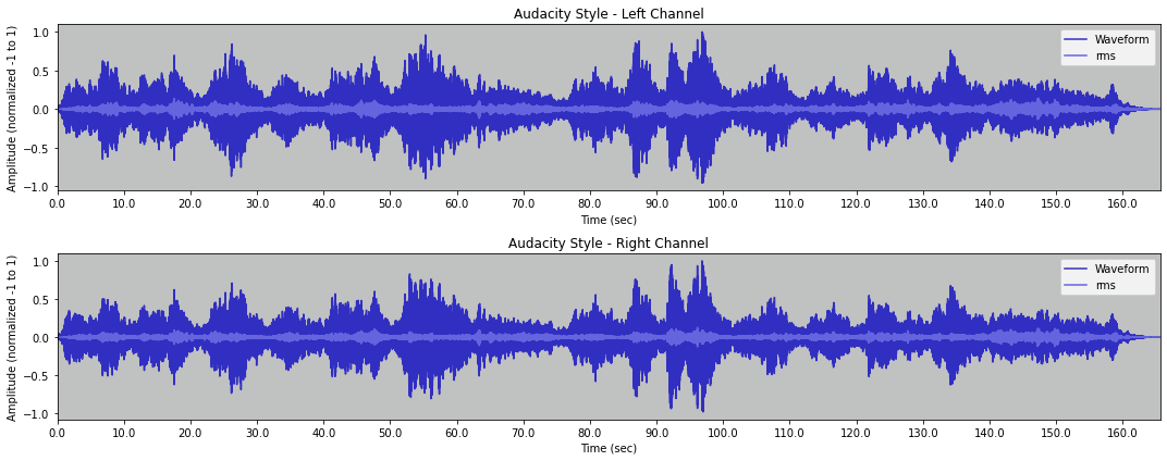
We then created some waveforms in different styles, allowing us another view on the musical information of our piece. We wanted to visualize the frequency content of the stereo waveform, so we created 6 new waveforms from the originals and discarded any frequencies above, between, or below two thresholds (one between high and mid, the other between mid and low). Low frequencies are coloured red, mids are green, and blue represents high frequencies relative to the frequency content of the file. There is little blue in this plot because there is little to no audio information in the highs of the audio input as defined by our program. The light green areas are overlaps between red and green. Three tracks for each channel were then layered on top of each other to show which parts were predominantly bright, mellow, or dark in relation to time.
Another way we visualized the audio was through layering the waveform with its own RMS, which gives a more accurate representation of loudness over time.
Informed by Information
So what do the many different ways of representing musical information digitally enable us to do? We hope that through our project we’ve shown that through synthesizing many sources, it is possible to get varying views and perspectives on a musical work, and to continue on to create something new, beyond what is possible when only considering a single source.