Introduction

Being students at the MCT program is now a condition we’ve gotten accustomed to as our first term is gradually coming to an end. Usually we get some sort of assignments to solve every week, and most likely we will spend way too much time solving it. So when the last assignment was announced we decided to get extra ambitious and spend even more time on it, making sure our personal lives and sanity would be completely ruined come Christmas.

We decided to use our recently acquired Python skills to build a program that could mix a multitrack recording. With homebrew FX and everything you’d need, basically making a tiny Python-DAW except for a nice GUI. That would have made it too slick, we wanted this to be pure code.

The code for this project is available here.

The Music

In order to mix anything, we needed some music. And as our sanity was already slipping, we skipped this part until we had a program up and running. When time came to create the music our minds was so entrenched in lines of code that we almost had to write a Python program which could write music for us.

The solution was to pick some files from an old unreleased project of Arvid’s band Misha Non Penguin, and then take away all processing and writing them out as mono files.

We ended up with five tracks:

two drum tracks
one bass synth
one synth brass stabs
one plucked lead synth.

On purpose we chose poorly sounding synth patches, completely unprocessed. We also had a midifile containing all the midi. The challenge was on.

The original unprocessed music

The Program

Segmenting and rejoining segments of audio has somehow become the bread and butter of the MCT program, so the assignment required us to do this. But this was also going to enable us to apply different processing on each segment of any track, which turned out to be an interesting option in the end result.

The basic thing needed whenever things are sliced up and pasted back together are some short overlap and fading functions, in order to avoid clicks and artifacts in the sound. Our approach to achieve this was the following:

Creating an empty array of zeros called results, with the same size as the audio we’d segment.
Running the audio file in a for loop
Based on MIDI which gave us the downbeat of every measure, we would slice out one measure of the audio.
The segment would be given a short fade in and fade out (equal to the length of our overlap, see further down)
This segment would then be processed with whatever effects we wanted.
The segment would be zero padded (adding zeros) in the front of the segment and in the back, making the segment the same size as the original audio and our result array.
Finally the segment would be cut in the beginning by an amount equal to our overlap (set to 1024 samples in this project) and zeros were added in the end to make up for the samples removed in the beginning.
The overlap value would then be updated for the next loop, in which it had to be equal to it’s former value + itself in order to work.
Eventually we would sum the result with the segment, and repeating this process until the whole track had been mixed.

We’ll come back to this gloriously inefficient way of processing audio later, but whenever we refer to our for loop from now on, this is what we are talking about. As an example it could look something like this:

# Creating the result array we will add all signals back into
result = np.zeros(s.size)

# Temporary arrays used in the for loop
segment = np.array([])
seg = np.array([])

# Setting parameters for the loop
counter = 0
current_beat = 0
overlap = 0
overlap_length = 1024


for i in downbeats_sample_time:
    # To check computational time and where it struggles, uncomment print(i).
    #print(i)

    counter += 1

    # Slicing the segment from current_beat to the sample position i
    seg = s[current_beat:i]    
    # adding fade ins and outs to the segment
    segment = fade(seg, overlap_length)

    # Processing segments one by one with different FX and signal processing
    if counter == 1:

        segment = compressor(segment, 0.3, 1, 1)
        seg_fx = IRDelay(segment, 8)
        segment_padded = padder(segment, s, current_beat)
        segment_fx = padder(seg_fx, s, current_beat)

        segment_padded = (segment_padded + segment_fx)

    elif counter == 2:
        segment = compressor(segment, 0.3, 1, 1)
        segment = softClipper(segment, 7)
        segment_padded = padder(segment, s, current_beat)

    elif counter == 3:
        segment = compressor(segment, 0.3, 1, 1)
        seg_fx = IIRReverb(segment, 20, 800, 0.78, 1700, 0.68)
        segment_padded = padder(segment, s, current_beat)
        segment_fx = padder(seg_fx, s, current_beat)

        segment_padded = (segment_padded + segment_fx)

    elif counter == 4:

        segment = compressor(segment, 0.3, 1, 1)
        segment = reverse(segment)
        segment_padded = padder(segment, s, current_beat)

    # updating the current beat for the next loop
    current_beat = current_beat + seg.size    
    segment_overlapped = segment_padded[overlap:segment_padded.size]

    # getting the size right again by adding zeros to the end:
    segment_final = np.pad(segment_overlapped, [0, overlap])

    # Increasing overlap for next round of for loop
    overlap = overlap + overlap_length

    # Just making sure the sizes are allright
    segment_final = sizecheck(segment_final, result)

    # Resetting the counter when it reaches 4
    if counter == 4:
        counter = 0
    # pasting the segments back in, one by one
    result = result + segment_final


# Plotting the original track compared to the result after mixing it
plt.figure(figsize=(8, 4))
plt.subplot(2,1,1)
librosa.display.waveplot(s, sr=sr)
plt.subplot(2,1,2)
librosa.display.waveplot(result, sr=sr)
plt.show()
hihats = result

ipd.display(ipd.Audio(s, rate=sr))
ipd.display(ipd.Audio(hihats, rate=sr))

Our Processing Tools

Our tiny Python-DAW needed processing tools, and we set about to program the usual suspects in a DAW. We would need compressors, reverb, delay, saturation and filters for EQ-ing. Easy! One week until deadline? No stress.

Compressors

How does a compressor really work? Not like our first attempt. Our first compressor went through every sample checking if it’s absolute value was above a set threshold. Then it would check how much the sample amplitude exceeded the threshold, and finally multiplying it with a hardcoded value below 1. This was done in a for loop which could be ran multiple times depending on an argument in the function. After the for loop it eventually multiplied the whole signal with a makeup gain, enabling us to first compress the peaks, then turning the whole signal up a bit. In theory this little thingy did everything a compressor should do, but it did it in it’s own very time consuming way.

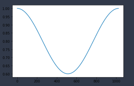
So it had to be improved, and that’s when we made our framecompressor. It uses a hanning window turned upside down as it’s compression envelope and analyses and compresses frames of the audio instead of sample by sample. We used a window of 2048 samples for our frames and then jumped back 1024 samples before analyzing the next frame in order to have some overlap and avoid pumping in the compression. It’s not too slow and did the job when we needed compression.

Upside down Hanning window with ratio set to -0.4, resulting in 0.4 compression at the most.

Reverbs and Delay

We made an IIR filter on the basis of Schroeder’s very first algorithm for creating an artificial reverberator.

It uses a set up of four parallel comb filters which then runs into two cascading allpass filters. Setting the parameters takes a little guessing and praying to the binary gods, and it’s not a reverb you would recommend to your favorite pop star, but it’s an actual reverb and we proudly used it in our mix.

Dry sound

Wet sound

Our delay was a FIR filter impulse response generating function, which does the processing in the frequency domain and therefore is much quicker to use. By choosing a number of impulses the audio signal would then be repeated as many times as the number of impulses, with a decreasing gain. It is definitely not an all purpose delay, as it works best on small segments of audio.

Brass stabs with our FIR Delay

Filters and saturation

For filters we chose to make a function that created a FIR filter which could be either lowpass or highpass, and which did the short time fourier transform (STFT) of the signal and applied it’s filtering in the frequency domain. This ensured it would be quick, and you could set parameters for passband, stopband and order of the filter in the arguments.

The saturation function (aptly named softClipper) uses numpy.arctan and some creative math to apply saturation (or distortion if turned up):

def softClipper(audio, drive, output=0.8):

    """audio = Source to be SoftClipped
    drive = Amount of SoftClipping (Try between 10-40)
    output = Output volume

    The signal is normalized before output attenuation for better control.
    """

    # Drive can not be set to 0
    if drive == 0:
        drive = 1

    piDivisor = 2 / np.pi
    driver = np.arctan(audio * drive)

    softclip = piDivisor * driver

    normalized = softclip/np.max(softclip)
    softClipped = softclip * output

    return softClipped

As the last of our fx we made a small function to reverse an audio segment. This maybe the only function that Python would do quicker and easier than it’s more user friendly counterparts. Just numpy.flip(audio) and the Beatles would have been sold.

Instruments

Our program also needed some instruments, or rather functions that could create sound. Why? Because DAWs have that. And we wanted to make a DAW in Python. Did we use any of them? Hardly. Just one of them. But it’s there and maybe someone else would one day feel the need to enter the abyss of doom and attempt to use our program to mix some music.

We made sine, square, sawtooth and triangle oscillators, and even a pulsewidth modulated oscillator with it’s own LFO. There’s also an ADS amplitude envelope.

Mixing the music

With our Python DAW up and running, we set about to actually process the audio files. At this point of time our deadline was a point in the distant past and sleep deprivation had kicked in, but the joy of mixing in Python kept us going through the night for a couple of days in a row.

The process would be something like this:

Load one track using librosa.
Applying some filtering, reverb and saturation in the for loop. Maybe set up some conditional processing or change parameters in a FX every time the for loop iterated.
Hit the run cell command in Jupyter notebook and wait for a couple of minutes before finally hearing the result.
Changing some parameters in the FX.
Repeat process from 3.

It might sound like a walk in the park but don’t be fooled. The computation would be deadly slow for some of our FX, and it could take hours of testing until we would achieve anything close to a pleasing result. Sometimes we’d get lucky and find some nice settings for our FX early on, while most of the time it would sound disastrously bad and require endless fiddling with the parameters and waiting for the code to run.

But at last you could end up with something interesting, and then say some prayers hoping it would work in the final mix.

Pluck synth unprocessed

Pluck Synth processed by our tiny Python DAW

Music visualization

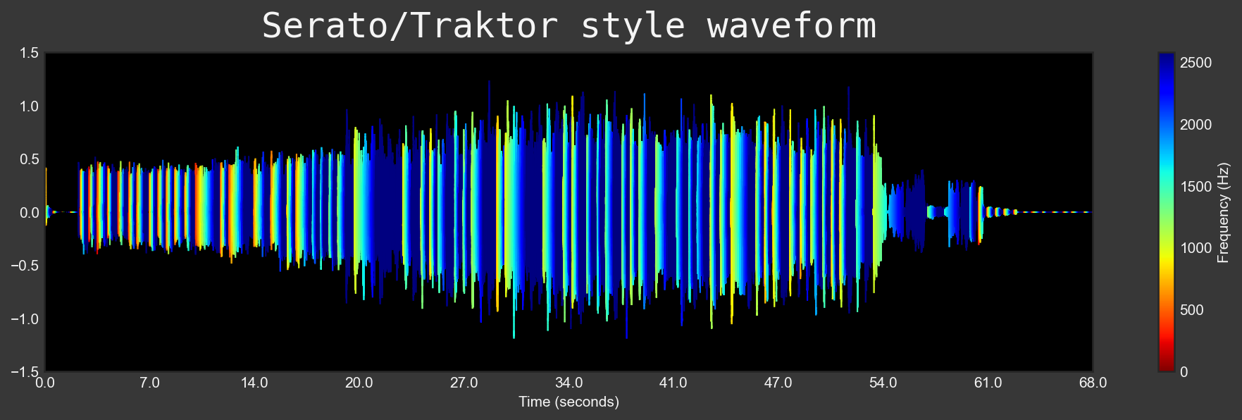
Finally, all we needed was a nice visualization of our waveforms freshly processed… Based on the most popular DAWs GUI, we could generate two waveforms style:

one similar to Audacity (with RMS & waveform overlapped)
one similar to Traktor/Serato DJ software (with vertical lines of the waveform color-coded by spectral centroid)

To acheive this, we first had to design spectral features functions based on mathematical formulas in order to extract the features we were interested in.

Root mean square, defined as the square root of the mean square (the arithmetic mean of the squares of a set of numbers).

${\huge RMS=\sqrt{\frac{1}{n}\sum_{i}{x_{i}^2}}}$

${n=\text{frame length in samples}}$

${x_{i}=\text{each frame}}$

Spectral Centroid, as the name suggests, a spectral centroid is the location of the center of mass of the spectrum. Since the audio files were digital signals and the spectral centroid is a measure, this appears useful in the characterization of the spectrum of our processed audio file signal.

${\huge Centroid=\frac{\sum_{n=0}^{N-1}f(n)x(n)}{\sum_{n=0}^{N-1}x(n)}}$

${x(n)=\text{the weighted frequency value, or magnitude}}$

${f(n)=\text{the center frequency of the frequency bin}}$

${n=\text{the bin number}}$

Furthermore, coloring a waveform with spectral centroid required that we

Compute an onset-detection function in order to locate note onset events by picking peaks in an onset strength envelope
Detect peaks in the onset-detection function to get the position of note onsets
Compute the spectral centroid over all the time segments delimited by the detected onsets
And finally, reshape the segments and time line values together and use a color gradient based on the range of the minimum and maximum centroid values of each segment

# Reshape the values for the plot
points = np.array([times, segments]).T.reshape(-1, 1, 2)
segments_reshaped = np.concatenate([points[:-1], points[1:]], axis=1)

# Plot multiple colored lines on the figure using line collection
norm = plt.Normalize(0, max(cents)/2) # normalize centroid frequency
lc = LineCollection(segments_reshaped, cmap='jet_r', norm=norm)
lc.set_array(centroid) # use centroid values to determine the lines
lc.set_linewidth(1)
line = ax.add_collection(lc)
cbar = fig.colorbar(line,ax=ax, label="Frequency (Hz)") # colorbar
cbar.set_label("Frequency (Hz)", color='#f4f4f4')
cbar.ax.tick_params(colors='#f4f4f4')

At last we could end up with something quite nice and informative.

the misty jungle — Coloring a waveform with spectral centroid

After a few nights of this ordeal we then had six tracks we could sum together. (We re-synthesized the lead synth with pretty midi’s built in synthesize() function, and applied our usual processing to the track in order to have two different lead synths which we could pan). We set different amplitude values for two tracks, the mixL and mixR, and then merged them together to form a stereo_file. And closed our eyes and felt asleep over our computers to the sound of our very own and very first Python DAW mix.

Our final mix