The Sound of Traffic - Sonic Vehicle Pathelormeter
Introduction
During the sonification Lecture series, we were exposed to fascinating concepts and theories behind sonification, sound design and their applications. Our primary goal was to explore the techniques that we learned and put them into practice in order to understand a real-world problem. After searching and referring so much available data we finally decided to work on traffic vehicle data from 3 regions in England measured over 17 years. Is it possible to transmit complex datasets within an instance of a sound, so the content gets revealed? As communication and dissemination of information in our modern digital world has been highly dominated by visual aspects it led to the fact that the modality of sound got neglected. In order to test the hypothesis, the project presents two prototypes for the sonification of temporal-spatial traffic data. While looking for similar projects, it was striking that ‘sonification of traffic’ is mainly applied for internet- and network traffic. In order to better comprehend data-streams and detect abnormal patterns for example. There is one project though with an approach very close to our experiment, found on LA-Listen by Steven Kemper. It extracts data from field recordings of moving vehicles and uses SuperCollider to generate Midi files aiming to use sound to further articulate patterns in the sonic data.
As stated earlier, we had been introduced with various facets of sonification from artistic and or qualitative approach like Øyvind Brandtsegg’s Flyndre Project or Daniel Formo’s Orchestra of Speech to a combination of both artistic and quantitative approach like sound examples by T. Hermann, A. Hunt and J.G. Neuhoff taken from chapter15 ( e.g. example #S15.3 ) from , The Sonification handbook (Hermann, T., Hunt, A., & Neuhoff, J. G., 2011) and so on. Our idea was quite like the latter approach. Hence, we decided to go for Parameter Mapping Sonification (PMSon) technique. In this technique, a data set is mapped with different parameter of sound synthesis which produce sound signals. Further, as per the definition of Sonification by Thomas Hermann (2008), a true sonification should have the following four attributes; (1) the sound should reflect objective properties or relation in the input data, (2) the transformation is systematic, (3) the sonification is reproducible, and (4) the system can be used with different data sets. Through PMSon technique, both of our prototyes meet these four criterias.
Data set
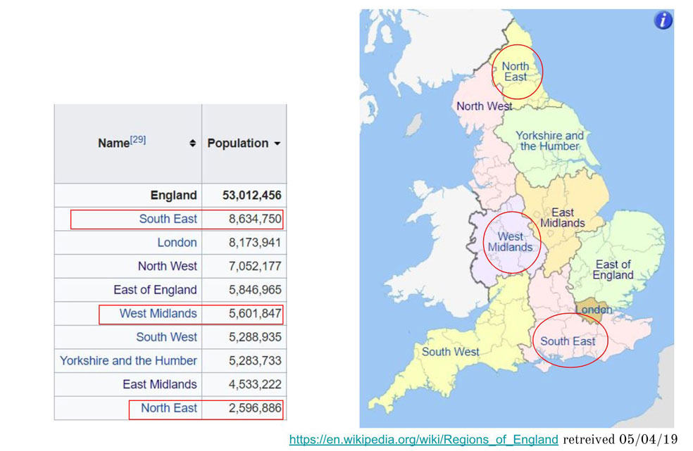
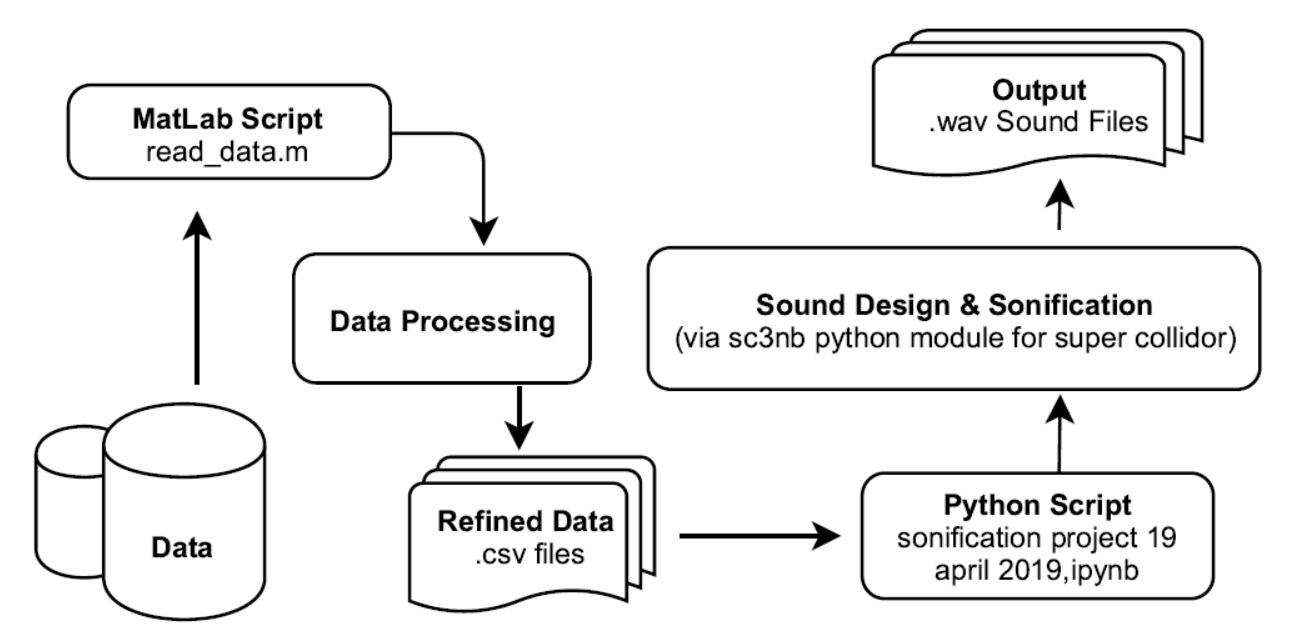
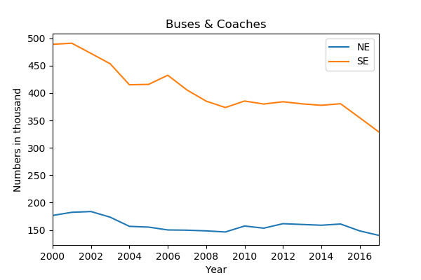
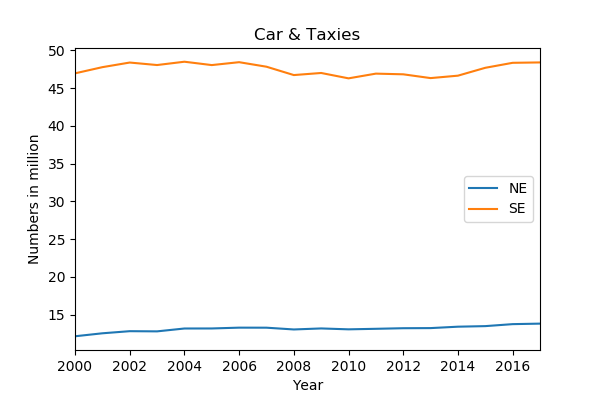
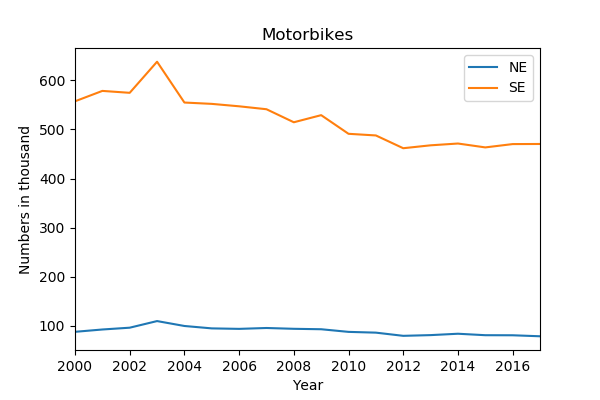
The data has been collected from The Department of Transport, U.K. It includes Annual Average daily Flow (AADF) of buses/coaches, cars/taxies and motorbikes for three regions of England from 2000 to 2017. The three regions include the North East, the West Midlands & the South East which have been chosen based upon their population as shown in Figure 2. The primary data includes number of vehicles, but they are segregated into numerous divisions of road types for each region. Shreejay made a matlab script to refine the data as per our requirement. The script reads the raw data of each region of choice at a time and writes them into an excel sheet by calculating the total number of vehicles in the region in each year and exports them as in CSV file format.
Sonification & Sound design
Prototype 1 with Javascript and P5.js
We chose to work with JavaScript to create our first prototype. The number of buses in each particular region was directly mapped into a frequency of an oscillator by using the “map ()” method in P5.js. Figure 3 below gives an overview of the mapping method. Here, for example, the minimum to maximum range of number of bus in each region is mapped to the minimum to maximum range of frequency.

Sound was generated through three unique oscillators that correspond with the data for each region. Additionally, three non-overlapping frequency ranges were chosen in the mapping to further differentiate between the three sounds. Moreover, the “settimeout()” method states the durations of a single frequency that corresponds to a certain year.
Code Snippet
The following code snippet shows how the three oscillators are defined and highlights the mapping method and set timeout () method applied in the prototype 1.
function preload(){
  loadJSON("Buses.json", dataReady1);
}

function dataReady1(data1){
  osc1 = new p5.Oscillator();
  osc2 = new p5.Oscillator();
  osc3 = new p5.Oscillator();

  osc1.setType('sine');
  osc1.freq(0);
  osc1.amp(0.4);
  osc1.start();

  osc2.setType('triangle');
  osc2.freq(0);
  osc2.amp(0.5);
  osc2.start();

  osc3.setType('sawtooth');
  osc3.freq(0);
  osc3.amp(0.2);
  osc3.start();

  figures1 = data1.figures;
  for (var i = 0; i < figures1.length; i++) {
    append(arrayBus, [figures1[i].AADF,figures1[i].NE,figures1[i].SE,figures1[i].WM]);
};

  // for three cities
  for (var i = 0; i < arrayBus.length;  i++) {
  setTimeout(function(y) {

    freq1 = map(arrayBus[y][1],140235, 183753, 200, 600);
    freq2 = map(arrayBus[y][2],227700, 377048, 700, 1000);
    freq3 = map(arrayBus[y][3],328924, 490877, 1100, 2000);

    //console.log(freq);

    osc1.freq(freq1);
    osc2.freq(freq2);
    osc3.freq(freq3);

    }, i * 500, i);
     // we're passing i
    };
  }
Prototype 2 with Python and Supercollider
The first prototype was further developed with Python and Supercollider. It is inspired by Thomas Hermann’s lecture on topics of Sonification and hands on exercise on Parameter Mapping Sonification during a series of talks in the MCT4046 Sonification and Sound Design course in this spring semester. The python code for this prototype is based upon two examples; Example-1: the code of the hands-on exercise provided by Thomas and Example-2: the code shared by Thomas through his GitHub repository. The code for the prototype has been further developed to adapt a different structure of data, create different synth definitions and apply different forms of mapping by exploring various example of synths in Supercollider. For instance, Example-1 and Example-2 have used synth definitions like SinOsc.ar, DynKlank.ar, Dust.ar etc while prototype 2 applies Saw.ar, LFPulse.ar and RLPF.ar along with combination of SinOsc.ar and so on. Moreover, the synths have been designed to meet our objective of combining both artistic and scientific approach, crafted in Supercollider, as shown in the code snippet below;
// ----------------Bus -----------------Amplitude & Frequency to be used in Mapping
SynthDef ("bus", {arg out=0, freq= 50, mul=0.7,amp = 1;
    var f;
    f = Saw.ar(freq,mul,0);
	Out.ar(out,f*amp);
}).add;

g= Synth.new(\bus)
g.free

// ----------------Car -----------------Amplitude & Frequency to be used in Mapping
SynthDef ("formula1", {arg out=0, freq = 2.5, mul2= 10;
    var f;
    f = LFPulse.ar(LFPulse.kr(freq, 0, 0.3, mul2, 200), 0, 0.8, 0.1);
    Out.ar(out,f);
}).add;

f= Synth.new(\formula1)
f.free

// ----------------Motorbike -----------------Amplitude & Frequency to be used in Mapping
SynthDef("motogp", { arg out=0, freq= 10, mul3 = 100, amp = 2;
    var m;
    m = RLPF.ar(LFPulse.ar(SinOsc.ar(0.2, 0, 0, 10),0.5, 0.2),freq,0.5,100);
    Out.ar(out, m*amp);
}).add;
m = Synth.new(\motogp)
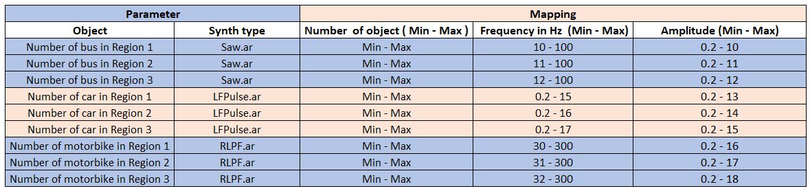
Similarly, Figure 5 below highlights the mapping of different parameters for the prototype 2. Here, for example, the minimum to maximum range of number of bus in each region is mapped to both of the minimum to maximum range of frequency and the minimum to maximum range of amplitude and so on. Therefore, for buses, the change in frequency and amplitude gives the idea of increase or decrease in number of buses in the selected region with respect to time. The speed of oscillation and change of amplitude signify the rise or fall of number of car/taxies in the region of choice with time. Similarly, for the motorbikes, the change in frequency and amplitude gives the information of change in number of motorbikes with respect to time in the selected region.
Code Snippet
import pandas as pd from matplotlib import pyplot as plt
d = pd.read_csv("Data_WM.csv")
import time, random, os
import sc3nb as scn
sc = scn.startup() # optionally use argument sclangpath="/path/to/your/sclang"
%%sc
SynthDef ("bus", {arg out=0, freqb= 50, mul=0.7, ampb = 0.2;
    var f;
    f = Saw.ar(freqb,mul,0);
    Out.ar(out,f*ampb);
}).add;
The code snippet above imports various python modules in the Jupyter notebook, required to make the sonification. Besides, it reads the data, boots supercollider using the sc3nb module and creates synth definition for buses and coaches using the Saw.ar synth in supercollider.
Similarly, the code snippet below sets TimedQueue function, which is required for creating sonification with precise timing. Synths are then initiated with a delay of 0.2 seconds and preparation are made for recording. Similarly, with iteration of the data, the algorithm maps the minimum and maximum range of the data to certain specified range of frequency and amplitude of the corresponding synth as explained in Figure 5. Finally, the sonification of each set of vehicle for each region is generated one at a time in wav file format.
queue = scn.TimedQueue()
t0 = time.time()
delay = 0.2

# instantiate synths
#queue.put(t0+delay, sc.msg, ("/s_new", ["bus", 1234, 1, 1]))
#queue.put(t0+delay, sc.msg, ("/s_new", ["car", 1235, 1, 1]))
queue.put(t0+delay, sc.msg, ("/s_new", ["motorbike", 1236, 1, 1]))

sc.prepare_for_record(0, "my_recording.wav", 99, 2, "wav", "int16")  # buffer 99 will be used
sc.record(t0+0.1, 2001)  # recording starts in 200 ms
#sc.bundle(0.2, "/s_new", ["car", 1234, 1, 1])
sc.stop_recording(t0+10) # and stops in 1 seconds

# modulate with data while playing through time
for i in range (len(d)):
    onset = scn.linlin(i, 0, 18, 0, 9)
    #b_freq= scn.linlin((d.iloc[i][4]), min(d.BusCoaches),max(d.BusCoaches), 10, 100)
    #print(b_freq)
    #b_amp = scn.linlin((d.iloc[i][4]), min(d.BusCoaches),max(d.BusCoaches), 0.2, 10)
    #print(b_amp)
    #c_freq= scn.linlin((d.iloc[i][3]), min(d.CarTaxies),max(d.CarTaxies), 0.2,15)
    #c_amp= scn.linlin((d.iloc[i][3]), min(d.CarTaxies),max(d.CarTaxies), 0.2,10)
    m_freq = scn.linlin((d.iloc[i][2]), min(d.MotorCycle),max(d.MotorCycle), 30,300)
    m_amp = scn.linlin((d.iloc[i][2]), min(d.MotorCycle),max(d.MotorCycle), 0.2,10)
    #queue.put(t0 + delay + onset, sc.msg, ("/n_set",
        #[1234,'freqb', b_freq,'ampb',b_amp]))
    #queue.put(t0 + delay + onset, sc.msg, ("/n_set",
     #   [1235, 'freqc', c_freq,'ampc',c_amp]))
    queue.put(t0 + delay + onset, sc.msg, ("/n_set",
        [1236, 'freqm',m_freq,'ampm', m_amp]))


# shut down synth when finished
#queue.put(t0 + delay + onset, sc.msg, ("/n_free", 1234))
#queue.put(t0 + delay + onset, sc.msg, ("/n_free", 1235))
queue.put(t0 + delay + onset, sc.msg, ("/n_free", 1236))
We bet you would also like to listen to the sonification of the third region of our second prototype and see full codes. Great! Just follow the GitHub repository and you will get access to all the sonification, codes, scripts, data files and other files related to this project.
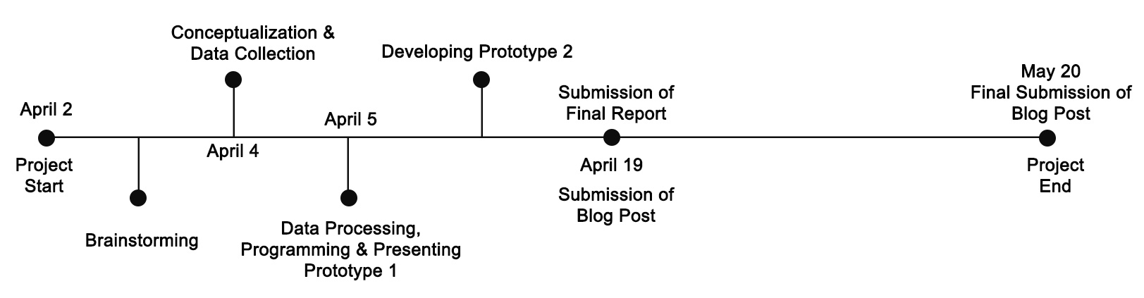
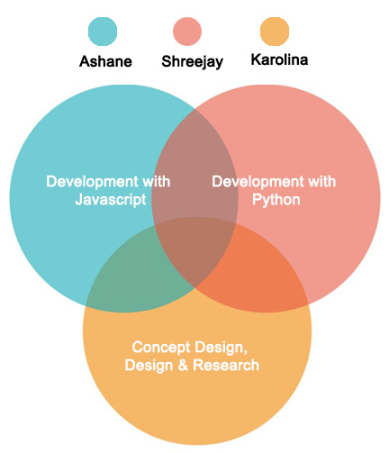
Project Timeline & Contributions
Main findings in brief
Prototype 1 was not revealing the actual content of the data. Although we chose non-overlapping frequency ranges in the mapping to further differentiate between the three sounds, it did not meet our objective of combining both artistic and scientific approach. Thus we decided to improve it and developed prototype 2. The informative qualities of the sounds, now standalone and representing each region/vehicle, could increase immensely. The structural elicitors like amplitude and frequency are creating again rhythm and tempo among others, which could reveal patterns in the content. In doing so it affirms our hypothesis.
Additional reflections
Our approach to perceptualize the data was from the beginning complementary, using sonification and visualisation. Especially together they have the power to convey information in ways also non-experts can comprehend. Going through the development processes of two sonification prototypes it posed questions how sound can be designed in order to become a standalone mediator of the sonified processes. Finally, the context of sonification and target audience refines the final outcome as well.
Future Work
Currently, the prototype 2 covers sonification of data for individual vehicle for a given period of time only. Running the sonification for the three vehicle types can mask each other and hide potential patterns of data. So, the sound design can be improved to make the sonification distinct as much as possible. Similarly, additional features can be introduced to the system such as the ability to select a preferred time period, to select certain transportation methods and regions etc. A data visualization tool can also be introduced to support the sonification model with multiple methods of visualizations to choose from. Another interesting suggestion appeared to build an API for sonification of traffic data of England, or any country with options for selecting different regions and different vehicles. The API could be extensively used for analysis and or for understanding the growth of traffic in the chosen region via sonification.
Acknowledgement
We are very grateful to Anna Xambo, our teacher for the MCT4046 Sonification and Sound Design course for exposing us to many experts and professionals working in the areas of sonification and sound design through this course. We would also like to thank her for guiding us in developing prototype 1. Similarly, we would like to extend our heartfelt gratitude to Thomas Hermann for sharing his plethora of knowledge on sonification. Likewise, we would also like to thank Thomas for providing us with his slides and python script and credit him for the prototype 2. All of them helped us practice, learn and expand our knowledge on sonification.
Thank you!
References
Hermann, T. (2008). TAXONOMY AND DEFINITIONS FOR SONIFICATION AND AUDITORY DISPLAY. 14th International Conference on Auditory Display, Paris, France June 24 - 27, 2008. Retrieved from: http://www.icad.org/Proceedings/2008/Hermann2008.pdf.
Hermann, T., Hunt, A., & Neuhoff, J. G. (2011). The Sonification Handbook (1st ed.). Berlin: Logos Publishing House. Retrieved from: https://sonification.de/handbook/.