Using convolutional neural networks to classify music genres
When classifying genres in music, CNNs are a popular choice because of their ability to capture intricate patterns in data.
So, how can we implement a CNN of our own? Well first of all, the key to any successful machine learning project is the data that we base our work on. For music genre classification, one popular choice is the GTZAN Dataset. The GTZAN dataset is a collection of 1000, 30 second song snippets, divided into 10 different genres. Perfect for our task.
The next step is to prepare each audio file to be used with our CNN. We don’t want to pass the CNN entire audio files. As you’ll remember, CNNs are effective on images. Therefore, we want to faithfully represent our audio data as image data. 2 ways to do this is by extracting the MFCCs-, or by extracting the Mel spectrograms of the audio files. For this project we will extract both MFCCs and Mel spectrograms, and compare the results when using either one.
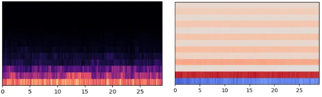
Example Mel spectrogram on the left, MFCC on the right To visualize the difference in MFCCs and in Mel spectrograms from genre to genre, I have added every MFCC and Mel spectrogram in each genre together and extracted the averages. For the MFCCs, every genre has it’s characteristics and nuances and some genres are more distinct than others. Metal is easily distinguishable from the rest with it’s blue rows, while classical also stands out with it’s almost undefined individual rows. The Mel spectrograms also has their nuances. Again, classical stands out with less activity in the lower frequencies than the rest of the genres.
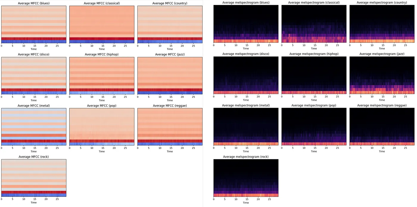
Average MFCCs for every genre on the left, Mel spectrograms on the right As we can see, there lies some differences in the MFCCs and Mel spectrograms from genre to genre, that our CNN will hopefully be able to pick up on.
Let’s move on to see how the program itself works. At the core of our program is the model. A single model can be trained on the dataset in less than a minute. One model is the result of many parameters and choices that can be tweaked and tuned to improve performances. However, doing this manually can be tedious. Therefore, we implement something called grid search to optimize parameters. Grid search works by defining a grid of parameters, simply put a list of parameters, each containing a list of values to choose from. Our goal is to find the best combination of values for every parameter. We can achieve this by working through the parameter grid in a loop, and keeping track of our results.
Already, we are training a lot more models. In fact, because we have 2 different types of features (MFCCs and Mel spectograms), 2 different types of CNN architectures and 2 different types of batch sizes, we end up training 8 models to find the ideal one. Already a substantial increase in training time, but it gets longer.
Whenever we train a model, we can get lucky and we can get unlucky. If we ran 8 models one day, we would probably not get the same results when running the 8 models the next day. Therefore we introduce something called stratified k fold. Stratified k fold allows us to re-run a model, with different portions of the audio files each time. In the case of our program, we run the models 5 times, and retrieve the average accuracy of every model. This serves as a much more reliable way to assess the performance of models. The trade-off is that the training now takes 5 times as long, in total 40 times as long as our original single model.
Now that we have the most important pieces of our program, let’s run it and explore the results. The first thing we are met with after training the models is this table:
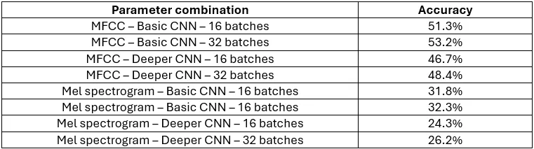
It contains all 8 combination of parameters, and their respective average accuracy. The first thing we can see is that in this program, using the MFCCs performs consistently better than using the Mel spectrograms. The second thing we can see is that the deeper CNN actually performs worse than the basic CNN. However, the accuracy is only a small part of the results, and doesn’t tell the whole story by itself.
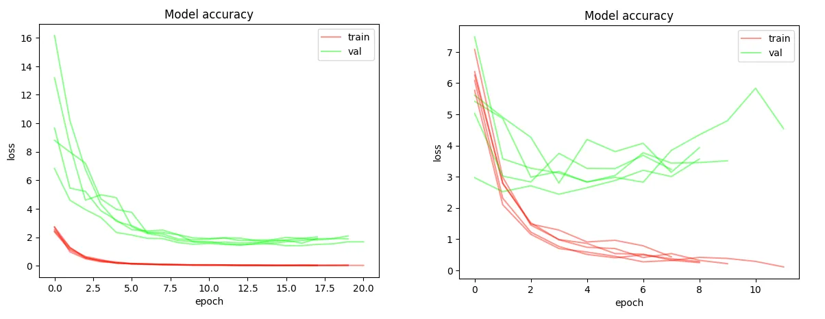
Loss function for best performing model on the left, worst performing model on the right Above is the loss function from the most and least accurate models. The loss function tells us something about how good the model’s predictions are. When the loss is low, the model should be able to consistently predict the right genre. One important difference in the loss functions is that in the least accurate model, the gap between the red training lines and the green validation lines grow bigger over time. This is a sign that the model is only improving on the exact data it’s training on. When presented with other data, the model will perform worse.
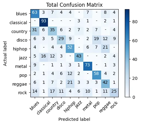
Confusion matrix for the models with the best combination of parameters Here is the confusion matrix for the best model. The confusion matrix simply shows what genres audio files are predicted as. There is a clear diagonal pattern, which is a good sign, but there are also many misclassified genres, leading to a less than optimal result. If we look at the individual genres, we can see that classical performs very well with a 92 % accuracy, followed by metal with a 73 % accuracy. These 2 genres also happen to be the most visually distinct genres if we look back at the average MFCCs and Mel spectrograms. On the other side, rock is the worst performing genre by far. It is one of 2 genres to be misclassified as every other genre at least once, and is consistently misclassified as country and blues.