Clustering audio features
Overview
The following blog post is about music information retrieval(MIR) and identifying similar patterns in my music library. I was curious to use unsupervised learning methods to analyze and cluster musical tracks based on their similar audio features. Generally, this approach can be quite helpful to increase the workflow of organizing musical libraries.
Features
For this example, the dataset consists of 50 wav audio files of the same durations, channel and sample rate. Usually, before we start the pattern recognition task and grouping sound files based on their content similarity, we first need to find a way to go from the low-level and voluminous audio data samples to higher-level representations of the audio content. This is the purpose of feature extraction (FE), the most common and important task in all machine learning applications. In my case, I aimed to extract the following features:
-
Spectral bandwidth - represents the difference between the upper and lower frequencies and has a direct correlation with the perceived timbre of the sound.
-
RMS - measures the average loudness or the energy of the audio
-
Spectral flatness - helps to differentiate between noise-like and tone-like sounds
-
Zero-crossing rate - classifies percussive sounds
-
Chroma stft - identifies pitch classes and melodic and harmonic content
-
Mel-spectrogram - approximates human hearing, as it emphasizes the lower frequencies more than the higher ones and provides the representation of the audio’s spectral content over time
-
MFCC - carries information about the sound’s timbre, phonetic content, and other characteristics
-
Spectral contrast - the difference between the peaks and valleys in an audio signal’s spectrum.
Clustering
After extracting features it is important to further preprocess data before feeding them to the clustering algorithm. One important step is feature scaling, which ensures that all features contribute equally to the distance calculations. This improves clustering results and accuracy. Also, it is especially important during k-means clustering, since it can be biased towards the variables that have larger values.
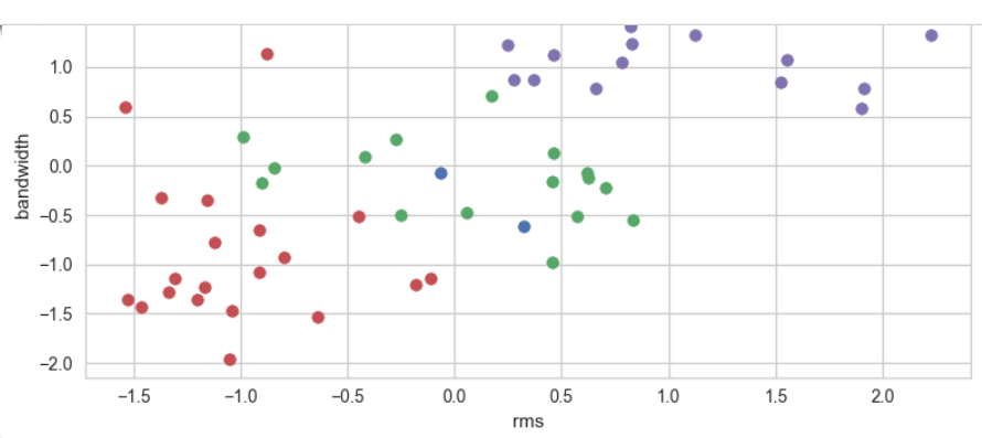
Then, I initialize k-means clustering algorithm with four clusters and a random state to fit the algorithm to the scaled features and generate integer labels for each data point. After selecting a specific cluster and retrieving the indices of the corresponding audio files we can display and playback the clustered audio files, showing their similarities.

Evaluation
During the evaluation of the optimal number of clusters in the dataset, Utilising elbow method and the silhouette score indicated that the system requires further refinement to improve the separation of the data points.
The elbow method revealed that the optimal number of clusters may be poorly estimated as the point of the curve is not diminishing steeply. Silhouette’s score of 0.4 suggests that data points are somewhat well-separated within their clusters, but there may be some overlap.
V Measure Score: 0.40947638495245836 Homogeneity Score: 0.43588570440829166 Completeness Score: 0.3860844120745334
All three metrics show that clusters do not contain data points that belong only to a single class and the number of similar data points that are put together by the algorithm varies.
