I trained variational autoencoders to generate a range of novel and authentic human whistling sounds. Surprisingly, while the capability of human whistling has been widely studied, it has not been focused that much using the power of machine learning until now. I was eager to see if this technology could capture the essence of whistling and create something truly unique. And the results did not disappoint! Join me in exploring the primitive beauty of whistling through the eyes of machine learning!

Data

I used MLend’s Hums and Whistles dataset, which contains recordings of people whistling different songs. I preprocessed the the dataset to get ready for the training.

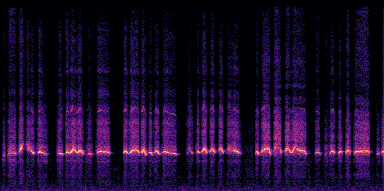
First things first, I min-max normalized the amplitude of the recordings. Then removed the silent portions that are over 500 ms, using the pydub library. To ensure smooth transitions, I added 50 samples fade in-out at the joining points. Next, I chopped each recordings into 65280-sample-long audio pieces, and disregarded the remaining slice. This awkward number is to make sure that resultant dataset has a power-of-two shape. I extracted spectrogram of each sample using librosa, on an fft window of 512 sliding 256 samples. Then, converted them to magnitude values.

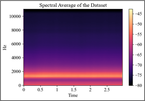
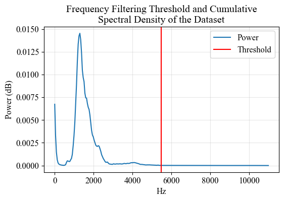
Next, I applied frequency filtering to the spectrograms to reduce their dimentionality. To do that, I started with analyzing the spectral density of the dataset to have an idea of the overall frequency behaviour of the whistlings. In that analysis, above 5400 Hz indicated no significant power and I decided to filter the frequencies that are not significantly used when whistling. The mentioned point luckily is very close to the mid-point of the frequency range, and I put a global threshold at the middle point (5469.4) to make sure things are in powers of two. Above I plot the spectral average and the spectral power distribution of the dataset, along with the filtering threshold.

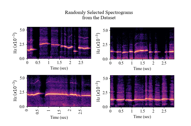
These steps resulted in ~12000 spectrogram representations with a shape of (128, 256). I splitted them into training and validation sets (80:20), and I was ready for training! See below the examples from the preprocessed dataset to have an idea of their shape and spectral behaviour.

Model and Training

After several experiments with different shapes and hyperparameters, here is the details of my final model desing.

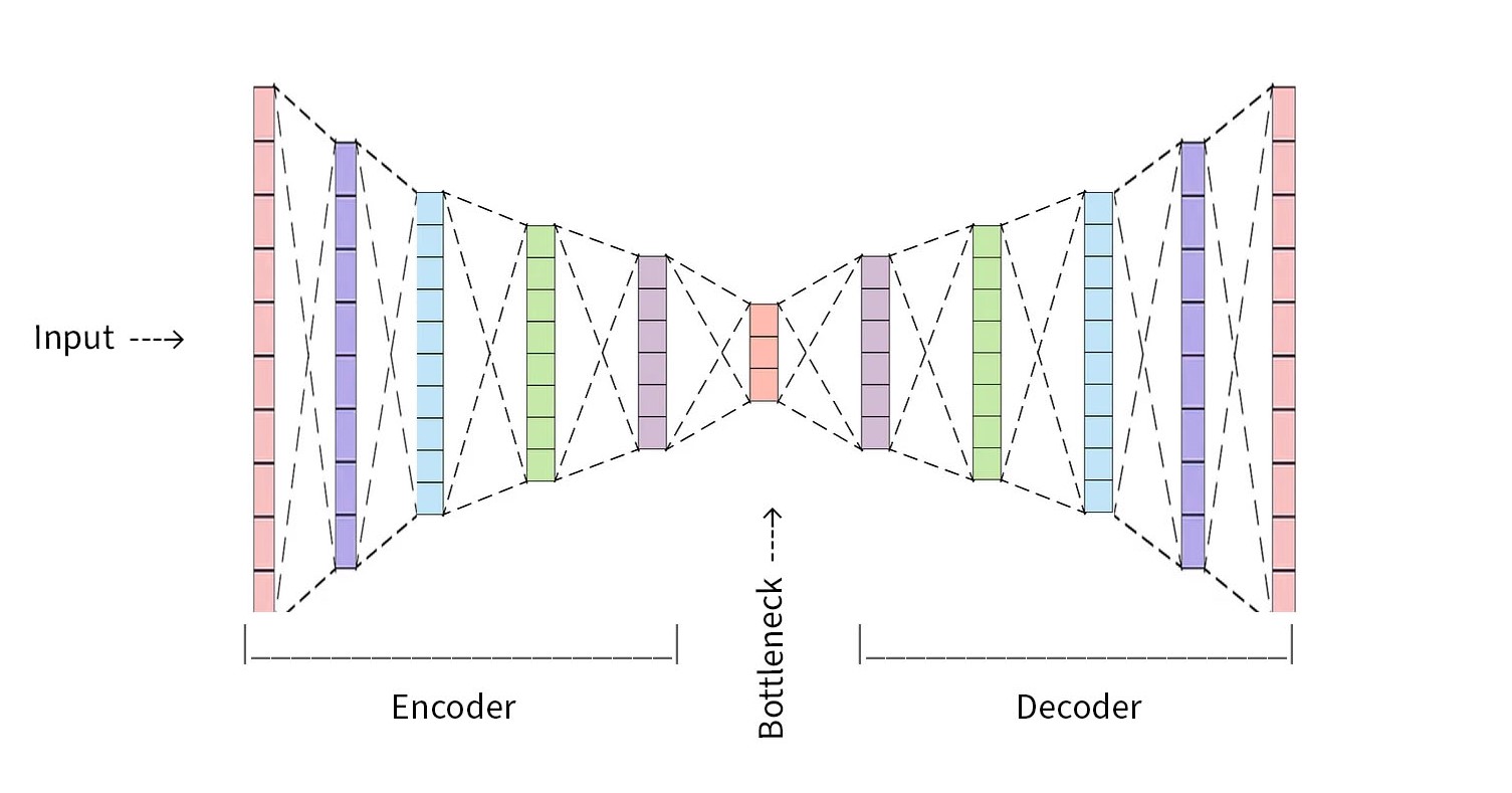
Encoder and Decoder

Encoder part has 5 convoltuional layers with 512, …, 32 filters. Encoder encodes the input spectrograms into a 64-dimensional latent space, by learning the characteristics of the spectrograms and mapping them as a probability distribution.

The latent space that encoder creates is a 64-dimensional array with spectrogram encryptions are scattered here and there. See below the UMAP latent space visualisation after the training.

Decoder part is a mirrored encoder, taking the encoded representations to reconstruct a spectrogram. Last layer of the decoder has a sigmoid function that produces a spectrogram output with values between 0 and 1.

Loss Functions

I used a combintaion of Kullback-Leibler Divergence (KL) and Mean Squared Error (MSE). MSE aimed to reduce the reconstruction error between the input and the output, while KL aimed to establish optimal probability distribution. I weighted the KL by $10^-6$ to balance their importance in the loss function.

Training

With all these, I trained the model with 10000 samples for 178 epochs with a batch size of 64. I performed the training on Google Colab, and it took around 3 hours with premium GPUs.

Generating New Samples

After training the model, I used the decoder part to generate new samples simply by randomly picking a sample from the latent space. Then, the decoder reconstructed a new spectrogram based on whatever it has in his mind(!) about the selected point. And that’s the final result, ALMOST!

Postprocessing

First I had to put the filtered spectrogram part back - I simply filled the missing parts with zeros. Secondly, I denormalized the amplitudes back to the normal range. Then I converted the spectrograms into audio using the Griffin-Lim algorithm. It is now a final result!

So what?

It went well! I think things worked and the resultant spectrograms are very close to human-made ones. Altough some noise in the background and some artifacts here and there, I could barely distinguish them from the originals. Also, worth mentioning that not all the generated spectrograms are that good - some were even terrible, sounding like an alien whistling, or someone practicing whistling while shaving.

Here are some generated whistling samples.

I will also conduct a user study with a pool of model-generated and original whistling samples. I will ask participants to rate the whistlings by their realism (in terms of audio-quality and expressiveness) to compare the model whistlings with the real ones. This way I hope to find out how unreal the model-generated whistles really are. I will add the results here when ready!

Keep on whistling and stay tuned!