Reverb Classification of wet audio signals
Machine learning is hard, and it takes a lot of time. It’s a lot of ups and down to figure out how to actually create a working program, or to find the data you are searching for. In this blogpost, I will talk about my trial of classification of reverberation times using machine learning.
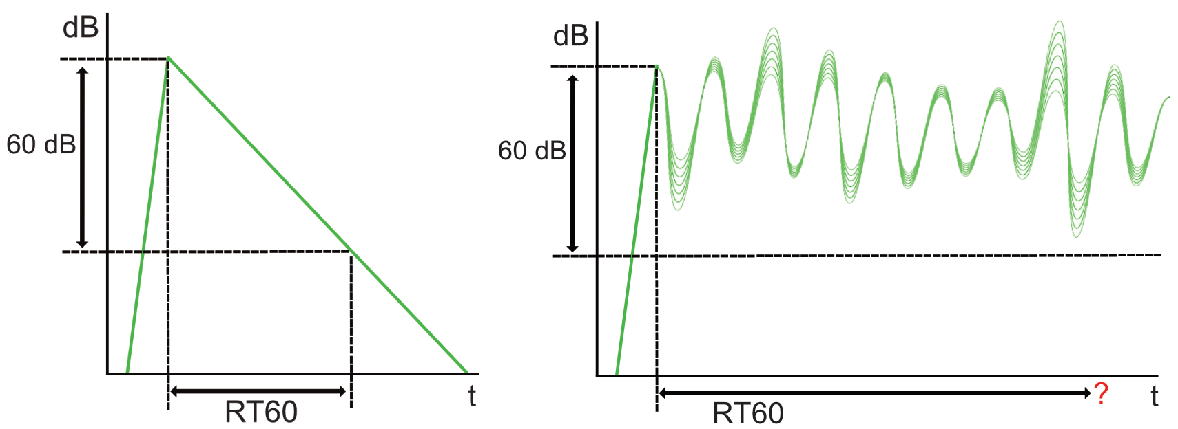
Classification of reverberation time is usually done by measuring a reverberant rooms RT60 value; the time multiple echoes uses to drop 60 decibels from the end of the transmitting audio. But when measuring a stream of continuous audio containing reverberation, this is not possible. Therefore, I wanted to see if it was possible to train a classifier using 21 reverberation lengths, applies to 100 random audio samples. Spoiler-alert: It did not work as intended.
The existing literature that seeks to predict RT60 vary in design. But the similarities in most of the systems are that most of them want to create a machine that can predict RT60 times from blind samples, meaning reverberate recording that the model has not seen. The most common papers found, was from researchers that participated in the ACE Challenge - Corpus Description and perfor- mance evaluation[1]. It is a competition to identify the most promising and non-intrusive Direct-to-Reverberant Ratio (DRR) and RT60 estimations in noisy reverberant speech. They offer a dataset that researchers can compete with, to accomplish the best RT60 and DRR measurements.
One paper that seeks to accomplish the ACE challenge [2] suggests that Attention-CRNNs are best suited for classification of reverb, where an attention vector is present in lower amplitudes of the signal, such as tails after peaks. As the other ACE-challenges, this is done on human speech and not music. In another paper [3], the authors hypothesise that using both temporal features in combination with spectral features is the best way to train a CNN to estimate RT60. Their results show that the estimation can be modelled as a regression problem and implement with a convolutional neural network. Their neural network outperform state-of-the-art algorithms form the ACE Challenge evaluation corpus for T60 estimation.
When looking at previous research that focuses on music related problems, one paper tried to match artificial reverb settings to unknown room recordings [4]. This can be a useful application, since matching organic reverberant recordings with artificial reverb is a time-consuming task. They have used MFCC as feature extraction, in a Gaussian Mixture Model (GMM). Existing recordings gets recommended reverberation settings from three selected plugins.
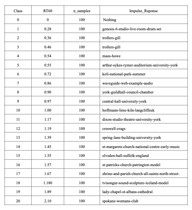
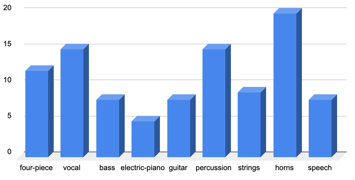
The database constructed had its main origin from the OpenAir library of impulse responses[6]. Choosing 20 suitable reverberations from their library of 100 impulse responses, was done on the basis of their length and general quality. The audio-samples was sourced from different dry audio signals mainly from the apples loops library [5], [7]. As we can see in the graph below, the 100 audio-samples was a large mix of everything available with limited reverberation. Other audio-samples were sourced from anechoic recording databases with high quality recordings. If you want to try this database yourself, you can find it here.
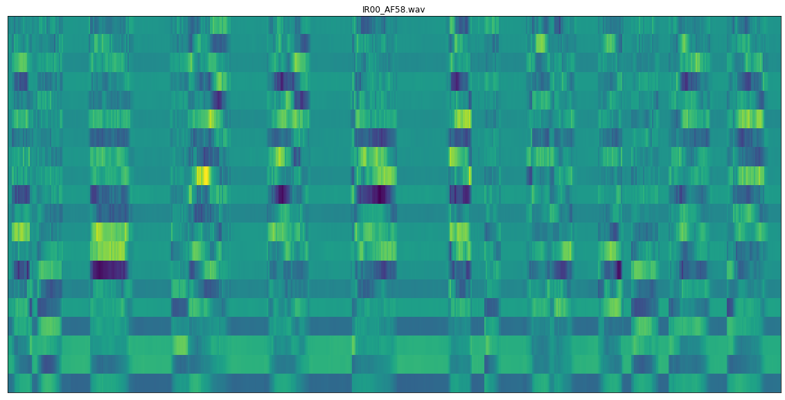
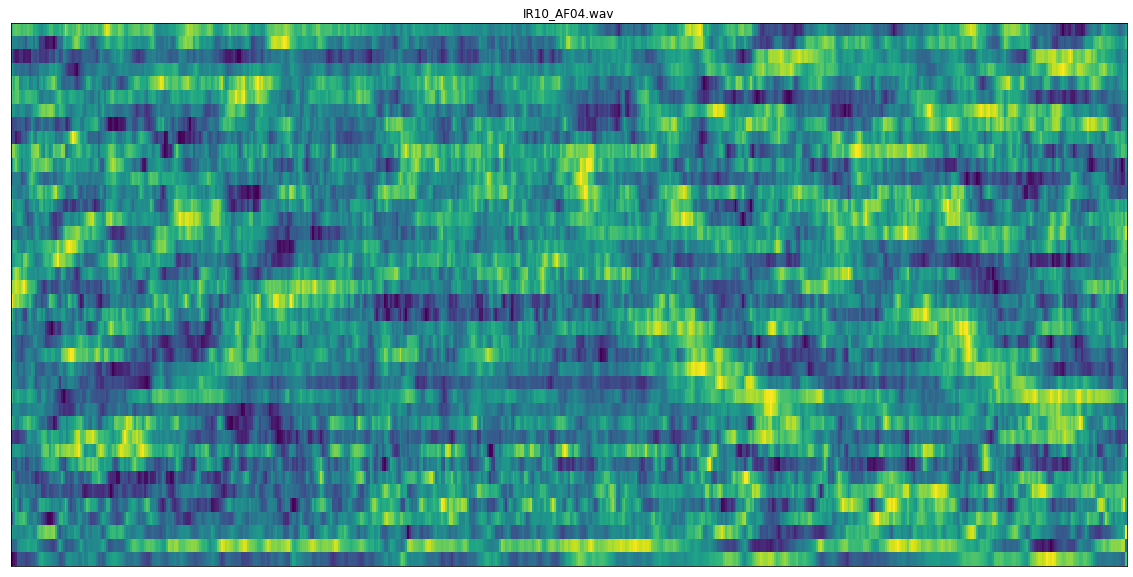
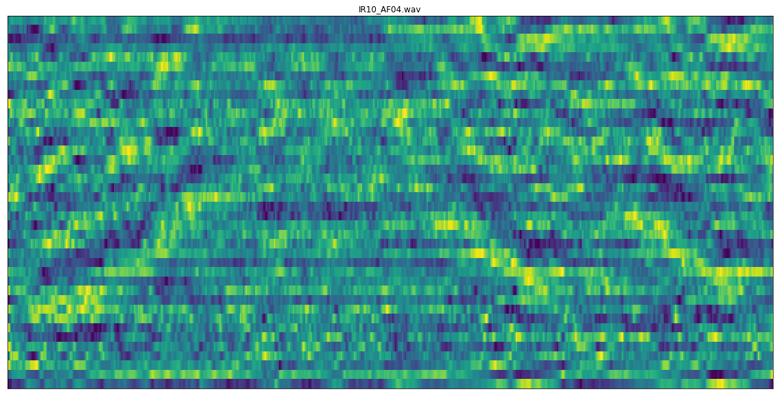
Feature extraction was done with librosa’s MFCC. Originally developed for automated speech recognition, it can be used as a temporal feature in music analysis. The chosen size of the MFCC was 40 mels, over a frame size of 2048 samples (42ms) and a window-length of 512 samples (10ms). The main problem with using MFCCs is that they are not robust to noise. Therefore a filter was applied at 400Hz to try to remove as much of the fundamental tones in the music as possible.
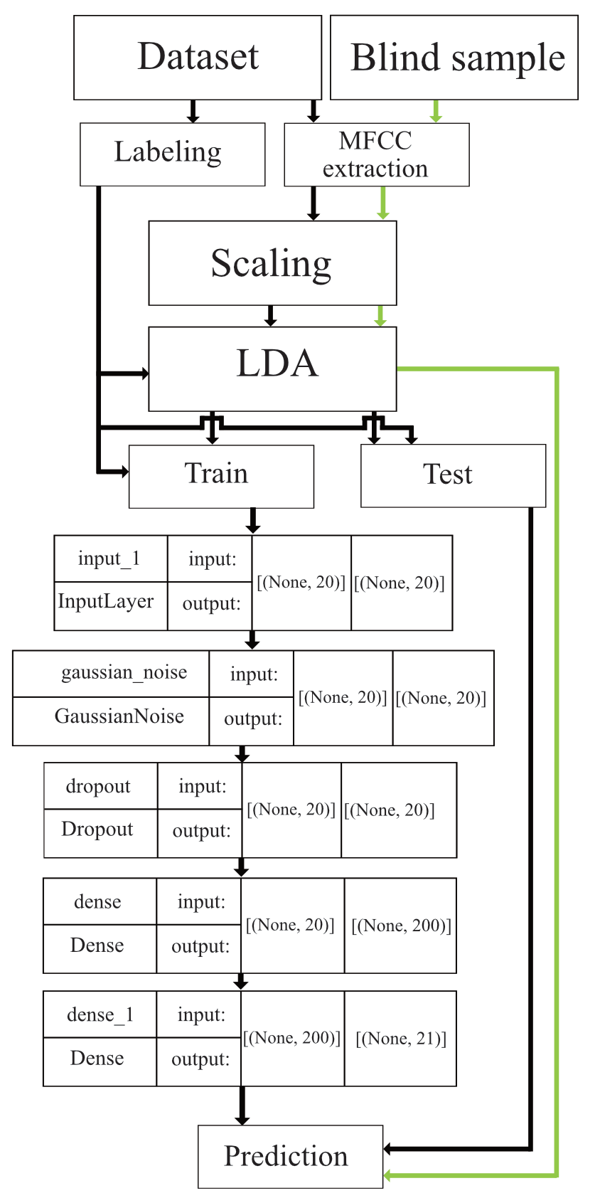
The model that I created had some flaws. As you can see in the diagram below, the LDA does most of the work. The tensorflow-model is trained on the basis of how the LDA is projecting the data, and the blind-samples was fed into the same transformation as the train-data. This is an issue when validating the data with the test data, since its projected in a way from the LDA where it already has been classified on the basis of the label given in the labelling-process (true label). The realisation of this fundamental issue came too late, mouthing in poor performance.
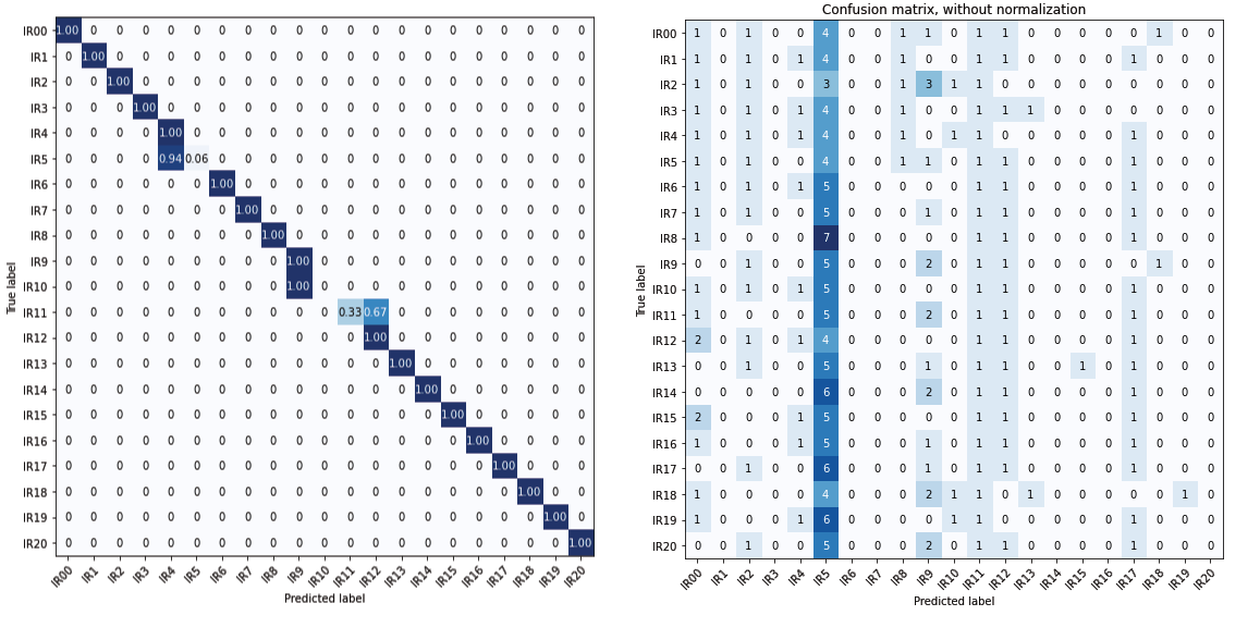
When running the LDA projection through a separate test-set with the same audio-samples that the model had seen, but different impulse responses, the model was able to predict the samples fairly well. But with blind samples that the model had not seen before that was similar but not the same, the model was not able to predict much. In diagram 4, we can se that the overfitting that happened in diagram 3 in class 5 is the fault for this.
In conclusion, the model created suggest that it is possible to differentiate between reverberation-times in wet audio-signal from monophonic instruments, opera, percussion, to quartets playing music together. But the model doesn’t work well with samples that is has not been trained on (blind-samples).
The model performs well when given impulse responses that are different from each other, both in length and in timbre. But with samples that are too similar, the model starts overfitting or under-fitting one of the similar classes. Compared to state of the art papers, this model is both of lower quality, and does not show the same results.
All in all, machine learning is hard. The joy of having a «working» model did that I didn’t validate the results. This lead to a later realisation that the model did not work at all.
References
[1] J. Eaton, N. D. Gaubitch, A. H. Moore and P. A. Naylor «ACE Challenge - Corpus Description and Performance evaluation» in 2015 IEEE Workshop on Applications of Signal Processing to Audio and Acoustics October 18-21, 2015, New Paltz, NY
[2] C, Papayiannis, C. Evers, P. A. Naylor «End-to-End Classification of Reverberant Rooms using DNNs» in IEEE/ACM Transactions on Audio, Speech and Language Processing Volume 28 2020
[3] H. Gamper and I. J. Tashev «Blind Reverberation Time Estimation Using a Convolutional Neural Network» in 2018 16th International Workshop on Acoustic Signal Enhancement (IWAENC)
[4] N. Peters, J. Choi, and H. Lei, “Matching Artificial Reverb Settings to Unknown Room Recordings: A Recommendation System for Reverb Plugins,” Paper 8700, (2012 October.) AES Convenction 133
[5] Apple, «Apple Loops Library» last modified 04 December 2022 https://support.apple.com/en-gb/ HT201907
[6] Open Air Library, «Anechoic and IR Data», visited 04 April 2022 https://www.openair.hosted.york.ac.uk/
[7] AVAD-VR «Audio/Video Anechoic Database», visited 04 April 2022 http://www.lam.jussieu.fr/ Projets/index.php?page=AVAD-VR