Emulating analog guitar pedals with Recurrent Neural Networks

Using a Recurrent Neural Network to model two analog guitar effects

As a music producer and guitarist, I love distortion. It’s a bit like champagne, it goes with everything. So for my Machine Learning (ML) project I chose to emulate two analog guitar effects using Recurrent Neural Networks (RNNs).
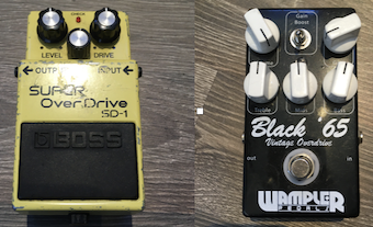
An analog effect is a non-linear system which changes some of the sonic characteristics of an audio source. The dry sound is input into the unit, and the resulting output is the wet audio. My chosen effects where the Boss SD-1 distortion pedal and the Wampler Black ‘65 tube saturator.

The Boss Sd-1 and Wampler Black 65'

Audio examples of a dry sound and how it sounds after being processed through the effects:

Dry Sound

SD-1

Black 65’

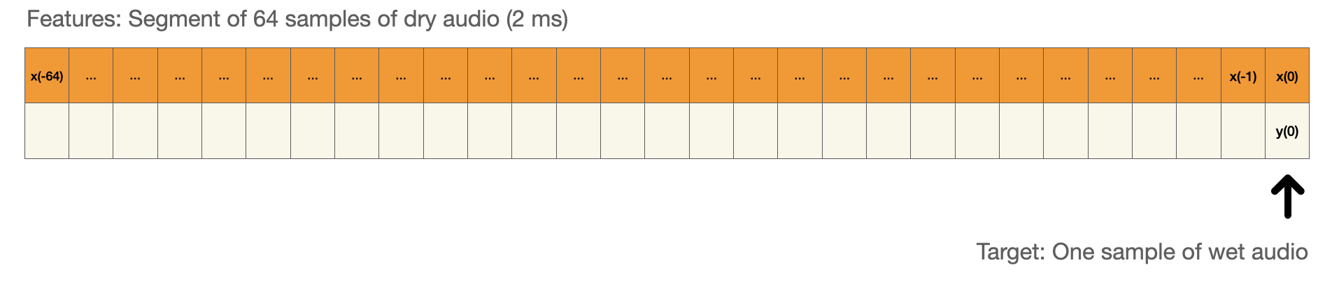
Using ML techniques, we are able to emulate an effect without having any prior knowledge of the effect we emulate. This is called black-box modeling. By feeding raw dry audio to a neural network, we can train it to predict the wet audio. More specific; we feed it a segment of dry audio and the model predict the value of the target sample of wet audio.

Frame of samples as input and one sample of wet audio as target output

Normal fully connected feed forward neural networks aren’t very good at this, because they are not able to keep any memory of former events. Even though my chosen effects had very short time-variances, they still affect the audio source in ways that needs to be understood in the time domain. RNNs are able to keep some memory of former events in their cell state which makes them quite good at learning how a non-linear system like an analog distortion effect works.
RNNs come in many forms, from the simple recurrent unit to the Gated Recurrent Unit (GRU). But the most popular and successful when it comes to audio effect modeling is the Long Short Term Memory unit (LSTM).

During my preliminary tests I quickly realized that the LSTM networks performed much better than the other RNNs. I also found that LSTMs had some peculiar challenges with audio prediction which I decided to explore. The result of this exploration was a comparative study of different LSTM architectures and different hyperparameters and how they performed modeling my chosen effects.

Dataset

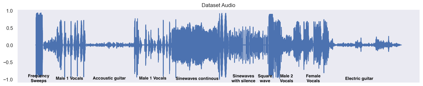
I created an 8 minute audio file consisting of different audio material. This audio was then recorded both dry and wet through my two effects. 20% of the recorded audio were set aside to be used for evaluation (The test set). The remaining 80% were the foundation for the dataset used for training the models.

The full dataset used in the project

Training the models

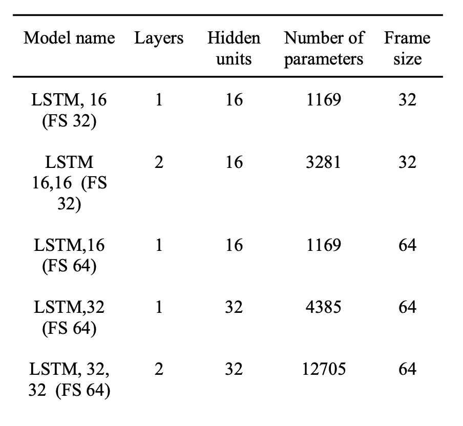
I made five different model structures, which has either one or two LSTM layers, 16 or 32 hidden units (inside the LSTM), and accepts as input either a frame of 32 samples or 64 samples. These different structures were then trained on different dataset sizes and different number of epochs, and compared to see who performed the best.

The five model structures.

Using Tensorflow with the Keras API, I trained hundred of models, and collected evaluation metrics from all of them which I used for analysis.
It took quite some time.
And every week or so I would come up with a tiny improvement and as a result I had to redo everything from scratch.

Results

To put it simple, the results can be explained this way:

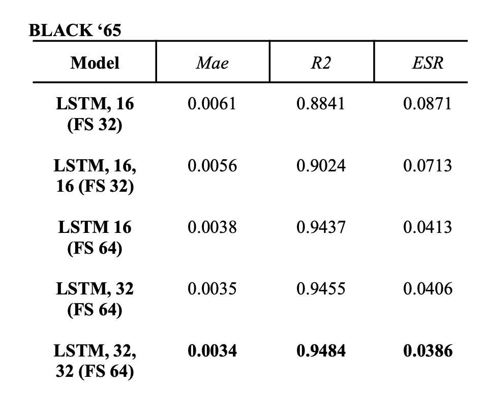
1. The models performed better on the SD-1 than the Black 65’ when we look at the evaluation metrics. But when you audition the predicted audio and the target output it’s hard to tell which effect is most similar.
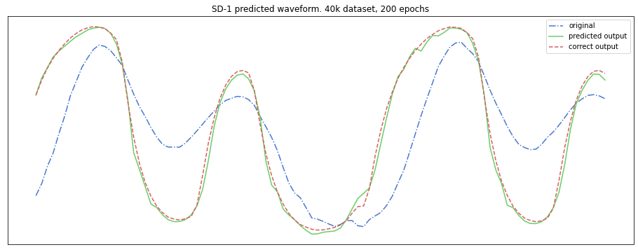
   (The following examples are one layer, 32 hidden units trained on 40k frames of audio.)

SD-1 True output

SD-1 Predicted Output

Black 65’ True Output

Black 65’ Predicted Output

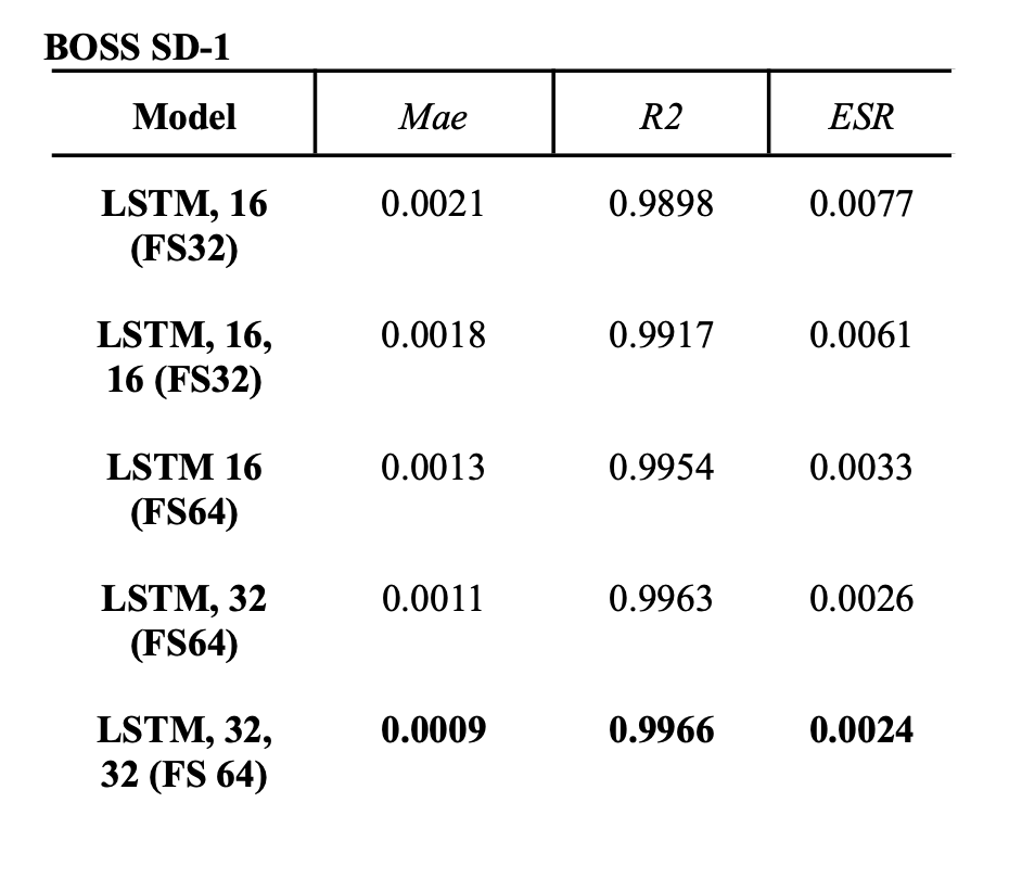
1. The bigger the model structure, the better the evaluation metric scores. Evaluation metrics are the Mean Absolute Error (Mae), Coefficient of Determination (R2) and Error to Signal Ratio (ESR).
2. The bigger the dataset, the better the evaluation metric scores gets. All the best performing models were trained on 500k frames of either 32 or 64 samples.

Evaluation metrics for the best performing models on the SD-1.

Evaluation metrics for the best performing models on the B 65'.

1. The evaluation metric scores do not necessarily correspond to my subjective perception of the similarity of the predicted versus the target output.
2. The longer the models train, evaluation metric scores improves, but the more they added unwanted high frequency material (noise and aliasing).
3. Visually inspecting spectrograms and waveforms often tells a different story than the evaluation metrics.

Waveforms of dry audio, target output and predicted output.

Noise and aliasing

In ML, an epoch is one training iteration through the whole training set. The number of epochs then determines for how long the model is allowed to train. Training for too many epochs can result in overfitting, or in the case of this project; noise and aliasing. Here you can see how the models first learn to emulate the low frequency content, then slowly learn to add the high frequency content. After 50+ epochs they start to add erroneous high frequent noise and aliasing artifacts. These examples were made with a dataset of 116 seconds of dry audio, rather small compared to the biggest datasets used for my experiments. However bigger datasets would cause the same behaviour:

Spectrogram of Target Output.

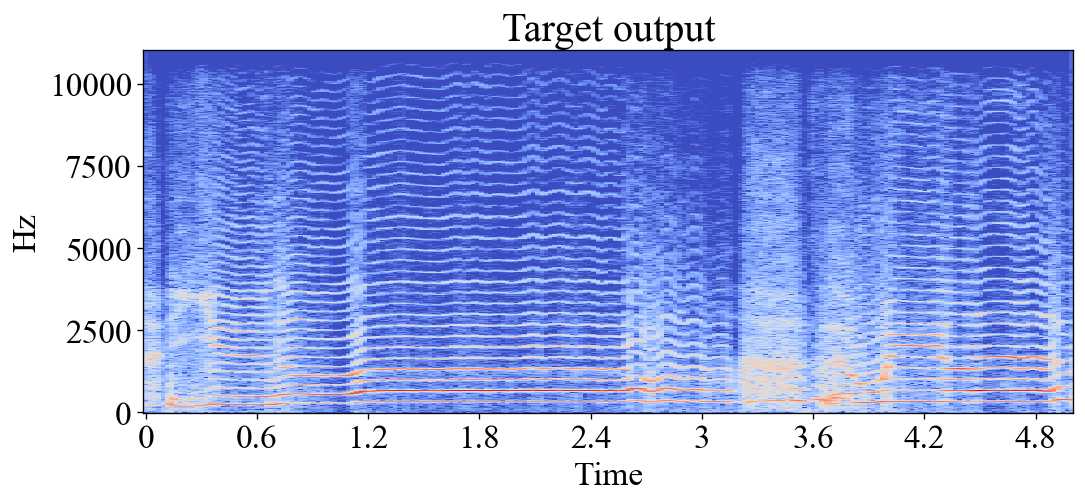
True output

Spectrogram of prediction after 20 epochs.

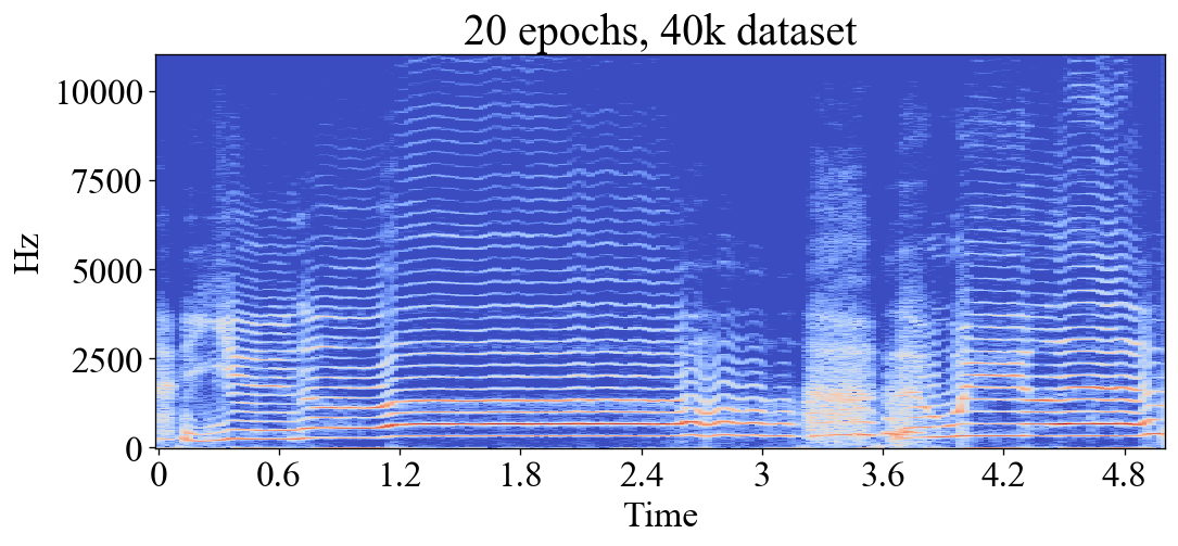
Predicted output after 20 epochs

Spectrogram of prediction after 35 epochs.

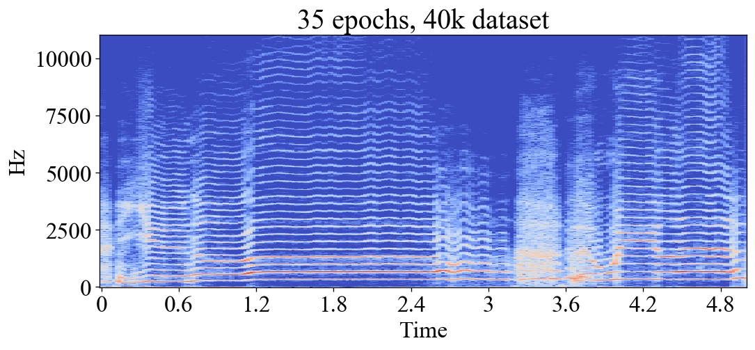
Predicted output after 35 epochs

Spectrogram of prediction after 50 epochs.

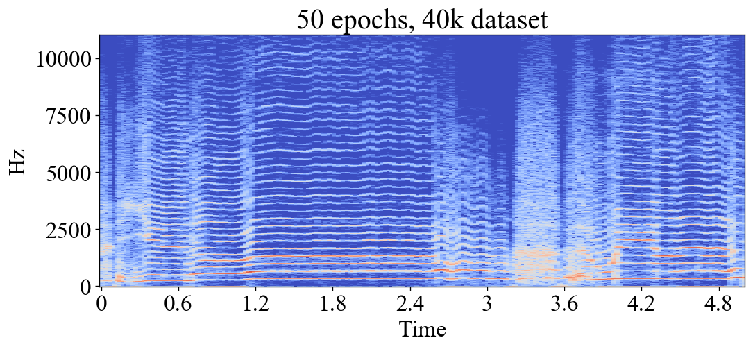
Predicted output after 50 epochs

Spectrogram of prediction after 80 epochs.

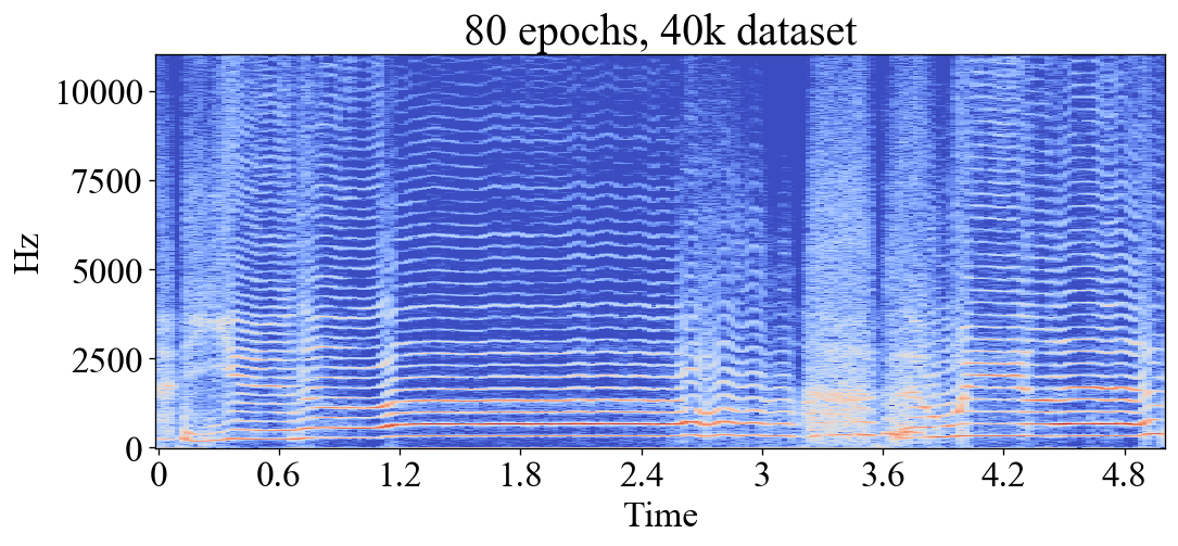
Predicted output after 80 epochs

Spectrogram of prediction after 200 epochs.

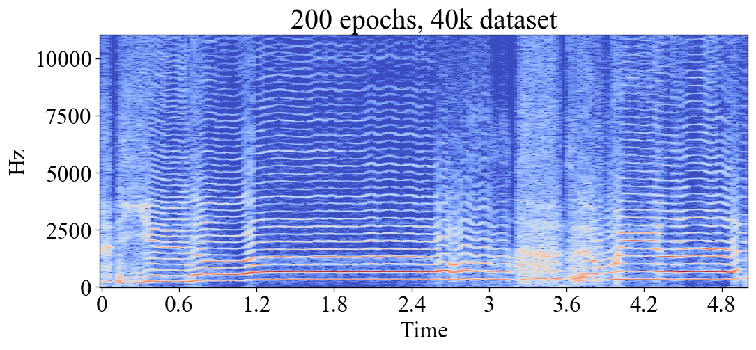
Predicted output after 200 epochs

This could however be because the LSTMs are doing a great job emulating the analog effects. All analog effects are non-linear, and non-linear systems will always produce content above the Nyquist Frequency, called the intermodulation product. Whenever audio goes through the process of Analog-to-Digital conversion, this is handled by a low pass filter filtering out the information around and above the Nyquist frequency. However because the high frequency content predicted by the models happens inside the digital domain, no such filtering is possible.

Takeaways

1. LSTM networks are pretty good at modeling analog effects with short time-variances. However they don’t work that well if the effect has longer time-variances (phasers, chorus) or memory (delay, reverb).
2. It’s hard to evaluate how similar a predicted audio signal is to its target audio signal. Evaluation metrics underestimate low energy high frequency information, in other words they don’t “hear” the noisy stuff.
3. Smaller and less computationally expensive models can produce pretty good results. The performance gain achieved by adding layers or more hidden units to a LSTM network are not necessarily worth it compared to the added computational cost and increased inference time.

The code for this project is available at Github.