Classifying Urban Sounds in a Multi-label Database
Environmental Sound Classification over Concurrent Samples
Given the short two week span to develop a machine learning model, I decided instead of beginning anew, to repurpose some pre-existing methods in approaching environmental sound classification. Environmental sound classification (ESC) is a field that benefits well from machine learning techniques, as the data examined will always be unique and noisy. Two well known databases, UrbanSound8K (US8K) [5] and ESC-50 [9] provide recordings from Freesound.org, trimmed, labeled and grouped into categories for analysis. This system attempts to utilise a convolutional neural network (CNN) on an augmented UrbanSound8K dataset for multi-label classification.
UrbanSound8K contains over 8000 sound files separated by categories of sounds typically found in an urban setting. Instead of exclusive categorical labels in its original state, the dataset has been recreated with the purpose of exploring how a successful architecture might perform on multi-label samples rather than simply uni-label, multi-class sounds. Thus, this project investigates how techniques in classifying an environmental noise database might generalize to a multi-label scenario with a new database composed of overlaid sound pairs.
The initial code that I forked was sourced from Aapid Saeed’s implementation which was in turn inspired by Karol Piczak’s 2015 paper that provides a scientific example of ENC using a CNN [4]. The experiment tested here provides some insight into the obstacles that appear when shifting this problem space both in terms of performance but also how features and parameters must be resituated.
Overview of dataset and fabrication
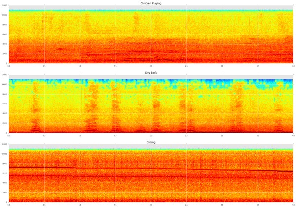
The original dataset, UrbanSound8K, contains 8732 .wav sounds sourced from Freesound.org across 10 classes of urban sounds:
- air conditioner
- car horn
- children playing
- dog bark
- drilling
- engine idling
- gun shot
- jackhammer
- siren
- street music
All are separated into 10 folds (each containing an equal distribution selection of the classes). These sounds are all less than 4s but vary in length, recording device, sample rate and perceptual loudness. Many of the sounds were generated as slices from longer sounds - meaning that many sounds share the same sound file source.
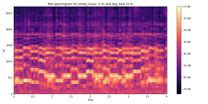
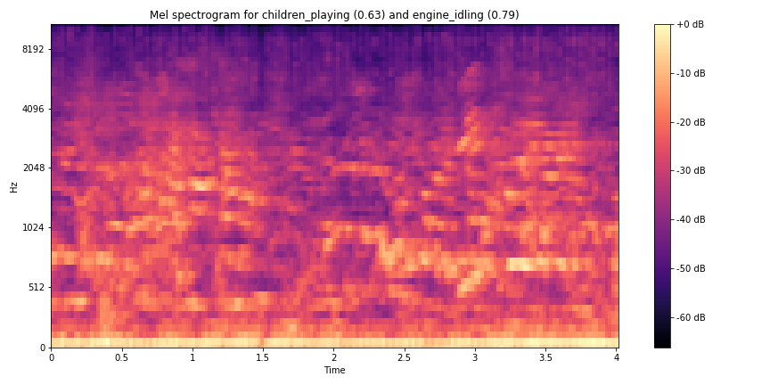
For creating a new dataset, I composed of multiple tracks of audio from UrbanSound8K. Using the library pydub, I created a separate script to use a randomized list of each fold’s files and overplayed each file with a randomized gain reduction between -6 and 0. This enabled a more authentic mixture of sound in a live context and would also contribute to the robustness of the model and its consequent difficulty during training (10 classes to 45 conceptual classes (or 10 choose 2)).
...
for j in range(multi_num): # number of samples to mix
    print(f'Processing: {samples[j]}')

    labels[j] = samples[j].split('-')[1] # get label
    sounds[j] = effects.normalize(sounds[j]) # normalize
    sounds[j] = sounds[j] + rand_gain[j] # add random gain reduction
    p_ratio[j] = pow(10, rand_gain[j]/10) # convert to power
    names[j] = f'-{labels[j]}({round(p_ratio[j],2)})' # label file with params

combined = []
combined.append(sounds[0].overlay(sounds[1], times=20)) # overlay sound (repeat if base sound is longer)
...
Two tracks of audio were chosen after testing the capabilities with three concurrent sounds, which appeared even too difficult to discern by ear - however, the script was written with the possibility of any number of overlays. This brings up another point - some of these classes of sound like ‘air conditioner’ and ‘engine idling’ closely resembled white noise, something that every recording ultimately contains due to the nature of recording sound. The final “multi” database is a little less than half the size of US8K as some of the samples of US8K were unreadable and were skipped.
Implementation of model
In addition to the creation of a script to fabricate and label a multi-labeled dataset, I augmented the scripts used to evaluate a CNN on the original UrbanSound8K database to suit this new multi-label scenario. The actual feature processing was identical to the one-sound-per-sample database. The audio data’s features (mel-spectrogram) were extracted and filtered with librosa.
Most of my efforts here went into changing how the labels were being processed. The network used to train and test the data was fashioned with the Keras wrapper for TensorFlow and other ML backends. Keras was chosen as it offers the ability to construcasdast neural networks at a lower level than the sklearn package whilst being fairly novice-friendly.
Model tuning for new dataset
Parameters that were previously provided by Saeed needed to be adjusted considering the new multi-label problem space. The first major change needed to happen at the label encoding level as labels were no longer a number from 0-9, an array of n values from 0-9. To resolve this, the labels were transformed into one-hot binary encoding. This allowed multiple simultaneous classes to be represented in an array of the same length.
Another major change concerned the end of the network, where predictions and evaluations are made on the training data. The final dense layer was set to the softmax activation function which was inappropriate for a non-exclusive multi-label scenario. The softmax function outputs probabilities for classes that sum to one, making it impossible for multiple classes to reach a binary activation. In this case, sigmoid offers probability distributions that are unconstrained, enabling multiple classes to reach binary classification.

In parallel, the loss function needed to be changed from categorical cross entropy to binary cross-entropy for this binary data.
Evaluation of performance
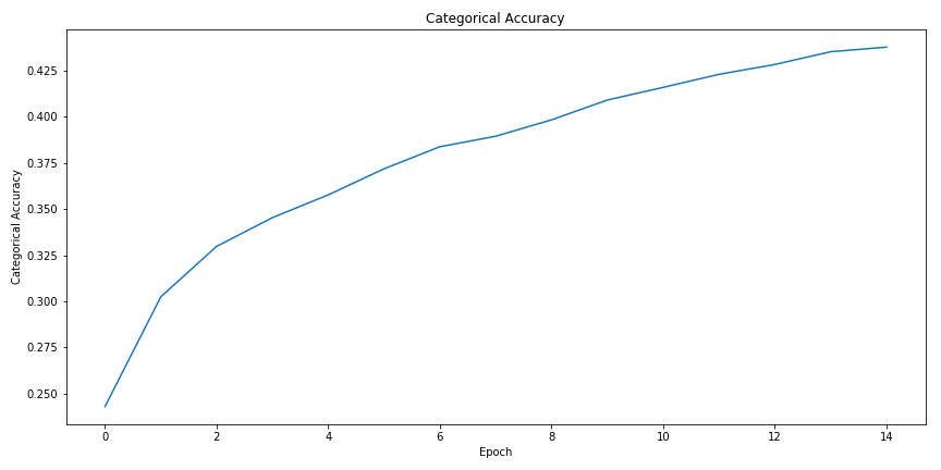
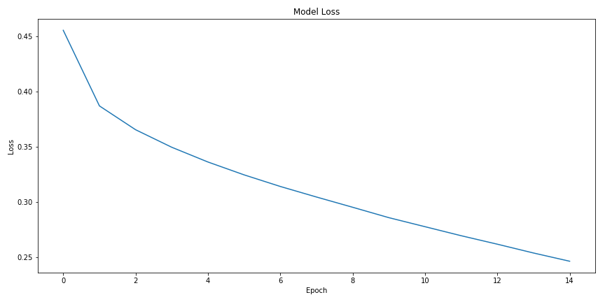
During training, the accuracy score increased to around 44% after 15 epochs while the loss continuously decreased. However, the last 10 epochs showed only a 4% increase in accuracy, suggesting the model was approaching convergence of the weight values and perhaps over-fitting (I had also attempted with longer training sessions with similar outcomes).
In testing the data, again the migration from a single categorical label to a one hot binary array means that the accuracy metric (a mean average of predictions on the test set) does not give us the whole picture. Moving to hamming loss, an estimate that shows use what percent of our answer’s elements were correct, is a much better metric when predicting on a multi-label sample.
The average accuracy was quite poor, as expected, sitting at 18%, however, the hamming loss (less is better) was 15%, meaning that 85% of the model’s label predictions were correct. These metrics are in sharp contrast to the performance of the untampered UrbanSound8K dataset, which was observed to have an accuracy of around 75-85% for most state of the art models [1, 2, 4, 8].
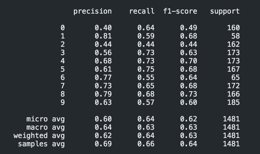
The confusion matrix and classification report, of one training instance, also provide interesting insights into how the test data was predicted. One major point to note is the time scale of some of these classes. It appears that those sounds that appear briefly with high impulses like the car honk, dog bark, and gunshot (1, 3, 6) are some of the most precisely predicted classes (low-false positives).
And as one might expect, the classes most difficult to label correctly turn out to be the noisiest and likely most organic and spectrally dynamic sounds within US8K: children playing, air conditioner and street music corresponding to 2, 0, 9. Of course, these metrics would need to be compared to the performance of the model on the raw UB8K database for one to make clear conclusions about how the shift into a multi-labeled dataset
Reflections
Not all of the details of the network employed have been fully elaborated and it may be that some transformations of the input data have been overlooked. Given the provided window of time and simultaneous introduction to techniques in machine learning, this investigation fulfils, at least, a tentative exploration into the field of ML based ENC.
One obvious challenge in mixing sounds as was performed in this experiment is the perceptual presence of the sound within the sample. This is actually accounted for by a subjective estimate in the taxonomy of the UrbanSound8K database where they determine if the category was a foreground or background sound. For categories like “air_conditioner” and “engine_idling”, poor classification performance would be expected when mixing sounds of these classes due to their lack of a sonic shape - they mostly consist of white noise. One might predict then that these categories were over-predicted on average across all sounds. Indeed, that does appear to be the case and this can be seen through the confusion matrix.
Another issue tied to the source database was its sheer size. The total time required to load around 9000 .wav files makes it prohibitively expensive when tuning parameters, or in this case, adapting the processing of files for a new problem space. K-fold validation would have been helpful in estimating the average accuracy of the model and providing greater confidence in our reflections of the model but there was not enough time to do so.
Code and instructions for setting up this project can be found here.
References
-
Abdoli, S., Cardinal, P., & Koerich, A. L. (2019). End-to-End Environmental Sound Classification using a 1D Convolutional Neural Network. ArXiv:1904.08990 [Cs, Stat]. http://arxiv.org/abs/1904.08990
-
Mushtaq, Z., & Su, S.-F. (2020). Environmental sound classification using a regularized deep convolutional neural network with data augmentation. Applied Acoustics, 167, 107389. https://doi.org/10.1016/j.apacoust.2020.107389
-
Piczak, K. J. (2020). Karolpiczak/ESC-50 [Python]. https://github.com/karolpiczak/ESC-50 (Original work published 2015)
-
Piczak, K. J. (2015a). Environmental sound classification with convolutional neural networks. 2015 IEEE 25th International Workshop on Machine Learning for Signal Processing (MLSP), 1–6. https://doi.org/10.1109/MLSP.2015.7324337
-
Piczak, K. J. (2015b). ESC: Dataset for Environmental Sound Classification. Proceedings of the 23rd ACM International Conference on Multimedia, 1015–1018. https://doi.org/10.1145/2733373.2806390
-
Saeed, A. (n.d.). Urban Sound Classification, Part 2. Retrieved 18 September 2020, from http://aqibsaeed.github.io/2016-09-24-urban-sound-classification-part-2/
-
Aaqib. (2020). Aqibsaeed/Urban-Sound-Classification [Jupyter Notebook]. https://github.com/aqibsaeed/Urban-Sound-Classification (Original work published 2016)
-
Su, Y., Zhang, K., Wang, J., & Madani, K. (2019). Environment Sound Classification Using a Two-Stream CNN Based on Decision-Level Fusion. Sensors, 19(7), 1733. https://doi.org/10.3390/s19071733
-
UrbanSound8K. (n.d.). Urban Sound Datasets. Retrieved 23 August 2020, from https://urbansounddataset.weebly.com/urbansound8k.html