Postcard from The Valley of Despair
The Setup:
Well, that was fun. Relax and have a good summer! they told us. And so we did. The trauma and triumph of the first year of MCT slowly faded as we road-tripped, climbed mountains, ran rivers, and leaped naked into fjords. We were children then, careless like the wind, our sunburnt faces besmirched with brunost and bringebær jam as we grilled waffles in the park (who does that?!) and washed them down with can after can after can of Who Cares pilsner.
And then, we came back.
MCT4047 is a tough course. There’s no sugarcoating it. Machine learning is a hard, bitter biscuit, dipped in cold data gravy. Eat and despair, ye who dare tread these shadowed neural pathways.
Or, maybe not. If you have a good background in maths, some programming skill, and a fully-functioning frontal lobe, it’s easy! How nice for you. As for me, all I can say is time will beat you like a rented mule. Add in a deep suspicion of robits and a pernicious latent Luddism in general, and I’m pretty much that old guy at the park shouting at the kids to get their damn computers off my park bench.
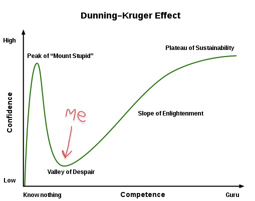
Figure one maps my approximate location on the Dunning-Kruger curve. I got over the peak of ‘Mount Stupid’ quickly, once the first week of MCT disabused me of any notions of expertise, and plummeted straight into the Valley of Despair. It’s hard to get out of that valley, especially without wheels (brains), but I’m doing my damndest, and occasionally some progress is made.
At least MCT4047 is well-documented, with extensive preparatory readings and hours and hours of video tutorials. Enough to keep you busy for years.
Except there’s a catch: you only have two weeks to prepare. Hahaha! Good luck, suckers!
An Attempt to Explain My Project:
I tried to come up with something reasonable, something I could get my mind around, something that wouldn’t compel me to fling anything precious into a volcano. A simple classifier or something. And so, I came across the Google datasets on spoken language. That looked fun, or something. Maybe I could discover something about the underlying musicality of language? Is that a feature one can extract? Well, we can try. Read on.
The Data Set:
I made a dataset by cutting down Google’s extensive set (like 18,000 examples) of short, spoken English phrases into 100 examples each in 11 different classes, making a total dataset of 1100 examples. Files were all 48kHz, 16-bit Wave audio. Six different regional dialects were represented, from Great Britain and Ireland, separated into male and female speakers. Intrepid readers who can multiply will note that there should therefore be 12 classes, not 11; apparently all the Irish gals were too busy takin’ a whirl ‘round the Salthill Prom with Mr. Earle to be bothered with this nonsense, so Ireland was only represented by the dudes.
To make the examples consistent, and therefore more palatable to The Machine, I used Librosa’s onset detection to trim the dead air from the start of each file, then set the duration to two seconds, the approximate length of the shortest file in the set. There, that only took me 37 hours.
The Features:
Features extraction is the most important part of Machine Learning in my opinion, which of course is completely meaningless. However, the features that one extracts from one’s data is what determines the success of one’s model, so choose poorly here and no algorithm will save you. ‘Garbage in, garbage out’, as my grand-pappy used to say as he ate gravy for breakfast. Those were his last words.
My thinking at this point was to try to get the algorithm to be able to identify dialects. This is what we in the Machine Learning space call a Classifier, a Supervised Learning technique in which we train the algorithm on a certain percentage of the data (usually 70-80 percent) for which it knows the labels (which classes are which), then turn it loose on the rest and see how it fares. When it performs better than random chance at determining the classes, we say that the algorithm has ‘learned from data’, and pat it on its ‘head’. Good algorithm.
Since audio files contain tons of data we don’t actually need for this task, we perform a process known as Features Extraction.
Let me see if I can explain. Let’s say we devise a system to distinguish Humans from Cats. We assemble a dataset culled from the most popular, trending images of cats and people on the internet. Now, we know that just because Harry Styles has four nipples, that doesn’t make him half an average housecat (or even two people), but our machine doesn’t know that. Especially if the only feature you extract from data is ‘Nipplegram’. Aside from the fact that this feature doesn’t exist in any ML library that I know of, apparently ‘number of nipples’ just isn’t a reliable predictor of species. Maybe we should try to detect the presence of fur. Wait, now Steve Carell and Zach Galifianakis are cats. Dang, this stuff is hard.
Or maybe those guys are just outliers. If your data set contains 100 images (way too small, what are you thinking?), and it classifies Styles, Carell, and Galifianakis as cats, and that one Sphynx skin cat with shy-nipple syndrome as a human, you still got 96 percent right. Hey, that’s pretty good!
The Algorithm:
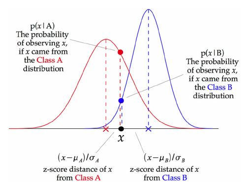
Oh, merciful science, there are so many. After dipping my toes into exciting-sounding neural networks like the Multi-Layer Perceptron and the encouraging Support Vector Machines, I settled on the aptly-titled Gaussian Naive Bayes classifier. It’s (relatively) easy to understand, if you understand Bayesian probability theory. Or, look at fig. 2. Pretend like you’re trying to find which category x falls into, A or B. Which curve does it go higher on? Bingo.
How the system performed:
So well! After K-fold cross-validation, my system returned an accuracy score of about 95 percent. It seemingly learned how to detect dialects, so I was successful, right? Nah. Going back to the dataset, I realized that the speaker within each class was always the same person, most likely using the same microphone, in the same room. The system was most likely detecting the unique sonic signature of a particular person’s voice coupled with their environment and the equipment used to record them. They could’ve been speaking Russian or Xhosa or gibberish and the results would have been the same.
Conclusion:
Back to the drawing board. See you in the Valley.