During these last two intense weeks of machine learning, I ventured to design a system that sought to recognize individual preferences in music using only the Spotify environment and API as resources. The model tries to predict the degree to which the author will enjoy specific tracks by Johann Sebastian Bach based on a subjective rating given to every example in the dataset. The dataset consisted of 100 Johann Sebastian Bach tracks collected from Spotify playlists. This unfortunate size of this dataset was due to the unexpected amount of time it took to gather music I liked (who knew?!). Anyway, the particular use of Bach’s works was not coincidental as it presented an opportunity to collect a relatively consistent body of examples in one particular genre (baroque) that I was familiar with.

The project was first and foremost aimed at exploring how a relatively new and accessible online resource of high-level musical data could be used for machine learning purposes but also to examine whether machine learning in this sense can be used as creative tools to gain new interesting knowledge about our personal music preferences and/or biases.

Data Collection

Collecting audio feature-data from Spotify was quite manageable due to their well-documented API. I decided to collect a variety of features for experimentation, including a few high-level features native to Spotify’s ecosystem; duration, energy, tempo, time signature, loudness, pitches, valence, danceability, timbres, key and mode.

Pitches
- The pitch feature returns a normalized vector per segment (a consistent subdivision of a track based on a consistent amount of sound) with 12 values representing the degree of occurrence for each note. I collected every pitch vector of a given track and averaged corresponding indexes. What remained was one list per track with the average occurrence of each note in the track.
Timbre
- Similar to pitches, the timbre feature returns a vector per segment with 12 elements. The specifics on what this timbre feature is based remains ambiguous, but it refers to the quality of the notes in the segment. The API also presses that these timbre values are best compared to each other. The gathering process here was the as with the pitch features.
Danceability
- This measure refers to how suitable a track is for dancing based on a combination of tempo, rhythm, stability, beat strength etc. Returns a scalar value per track.
Valence
- A normalized scalar of the “positiveness” conveyed by a track. The higher this value, the more happy, cheerful and euphoric the track is. The lower the value, the more sad, depressing and angry the track is.

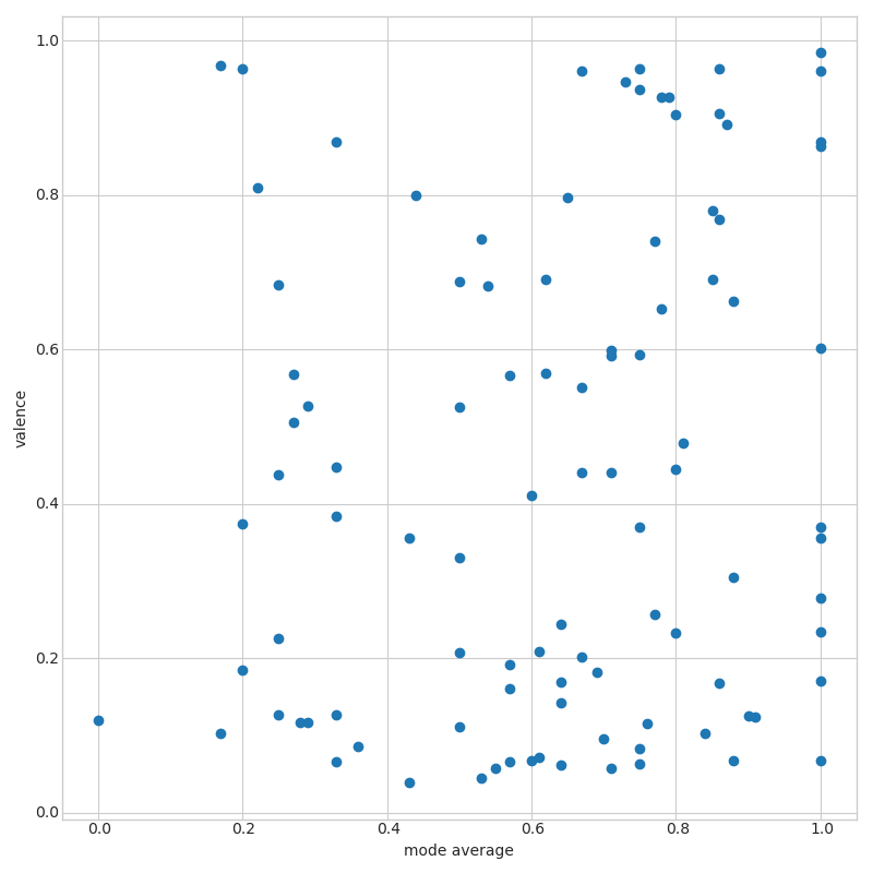
An interesting observation was that these high-level Spotify features did not immediately correlate with other suspected feature data. For instance, valence did not correlate particularly well with the mode of the tracks, as seen in the image below, something I anticipated.

Das Model

Since the goal of my project was to train a system to recognize my taste in music, a personal rating from 1-10 was given to each track representing target values for the supervised MLP (neural network) regressor algorithm intend. Additionally, I used a repeated K-fold for training and validation because I feared that more strict dependencies on particular percentages of samples in each target class, like what stratified repeated K-fold ensures, could be problematic due to my shortage of training data.

Both principal component (PCA) and linear discriminate analysis (LDA) were considered as dimensionality reduction techniques for the dataset. By comparing the variance of different sets of features to the total feature variance, I could find an approximation of how many reduction components I would need:

#Here we find the minimal amount of DR-components needed 
to keep 99% of the total feature variance.

feat_variance = np.var(features, axis=0).sum()
for i in range(features.shape[1]):
        temp = np.var(features[:,0:i+1], axis=0).sum()
        percentage = temp/feat_variance
        if percentage > 0.99:
            print("componenets needed: ", i+1)
            print("reached: ", percentage, "%")
            break

Even though the grid-search scores revealed a significant advantage of using LDA over PCA, I had to take into consideration that my system could be defined as a kind of hybrid between a classifier and a regressor. This is evident by examining the scalar nature and range of my target values. Therefore, the consequence of using LDA might be that it interprets my task as classification rather than regression, an interpretation that might compromise the validity of my algorithm. But even though PCA might have been more suited, its detrimental scores led me to use LDA instead and rather keep in mind the impact this might have on the model.

LDA cross-validation grid-search results:

best params: {'activation': 'logistic', 'hidden_layer_sizes': (2, 2), 'max_iter': 20000}
associated best score: 0.749

Lastly, the suggestion of using a logistic sigmoid activation function seemed logical considering that it’s often used to predict normalized probabilities which is exactly what my model would do.

Results

The general results were adequate and expected. However, with an R2 score of 0.75 on my limited dataset, I suspected signs of overfitting. In light of this, I conducted some tests by training the model on testing and training data before comparing the respective R2 and mean square errors. The larger the difference was between the comparisons, the more symptomatic my system would be of overfitting.

Original Training Data
Metric	Scores	Difference between training and test data predictions
R2	0.75	4-5%
MSE	-0.9	18-20%

As seen in the first table above, the first comparisons were not as bad as anticipated but still grounds for suspicion. To investigate further, I decided to artificially create more training data to test whether extending the size of the traing data could increase the performances and limit the metric differences.

Original Training Data + 1/4 Artificially Created Training Data
Metric	Scores	Difference between training and test data predictions
R2	0.8	3%
MSE	-0.7	13-15%

At best, I only managed to decrease the differences by approximately 2-3\% when adding 1/4 of artificial training data. The lack of performance variation from extending the dataset in this way can indicate sub-optimal algorithm parameters, dataset quality and/or dataset size. Most likely due to the latter..

Concluding Remarks

Evaluating performance metrics of a machine learning model depends on the system in question. I set out to prove that using Spotify data to train a machine learning model was feasible, and I believe this project has proved this concept.

The obvious dataset limitations were largely attributed to an inefficient process of gathering and labeling data. I believe that the system could have been better if the theme of the project was adjusted. For instance, comparisons of baroque composers or different musical genres could have facilitated a more effective data collection process. Alternatively, a more specialized focus, for instance on only piano sonatas or preludes, could also have yielded better results despite having a shortage of data.

For future work, it would be especially interesting to further explore and evaluate the high-level Spotify audio descriptors (danceability, valence etc..) through machine learning algorithms like this one.