Gyro-synth: A Musical Instrument Built with the Wekinator

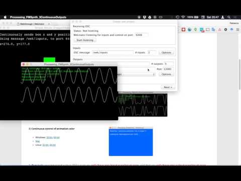
For the November 21st performance, our group trained a Machine Learning (ML) model using the Wekinator application to easily map a synthesizer with a mobile OSC controller. We used the gyroscope sensor in our phones and an FM synthesizer application that was included in the example applications provided by the Wekinator author. The gyroscope sensory sends three continuous data streams for the x, y, and z axes, and the FM synth had three input parameters for modulation, frequency, offset. The gyroscope data streams were sent directly to the IP of our PCs with the port and OSC message specified within the Wekinator program via two different OSC apps: Sensors2OSC for two of the members’ Android smartphones, and GyrOSC for the third member’s iPhone. The Wekinator, simply, is a software that makes the process of building a custom musical controller using ML easy and approachable (Fiebrink, 2010).

Here’s a brief intro from it’s developer, Rebecca Fiebrink

Setup

Once these apps were configured with each of our PC’s Wekinator applications, we specified the project parameters needed for our performance: port number, OSC message, 3 inputs, 3 outputs, output type as continuous, and model type as neural network. Afterwards, we chose unique parameters from the 3 outputs available within the Wekinator that would be mapped to the synth and would serve as our first training state. As a group, we first configured silence to the state of the phone held with the screen facing the user. The direct forward tilt was also roughly mapped to a different note on each device that would form a major chord when played together by all three devices. We then took these 5 recordings of 3-dimensional gyroscope data and trained (that’s “ML-talk”) the model using the Wekinator. Once complete, we were able to click “Run” and use our phone’s gyroscope as a controller to send both novel inputs to the Wekinator and produce novel outputs via the trained model’s interpolations.

The Wekinator then deploys a supervised learning algorithm on the labeled data we generate when recording OSC input messages while playing the FM synth. The model that we trained from this data was then able to predict a blend of these outputs even when receiving new data. The effect of this model allows us to have a continuous mapping of our synth to (virtually) any orientaton of our phones.

Performance

In our performance, we were able to achieve a level of expressivity and responsiveness that was able to be quickly achieved through limited training, and with just a few sonic anchors to navigate between. During our testing and evaluation of the configuration, we noticed that the continuity of the FM synthesizer’s parameters in response to the gyroscope was dependent on whether the labeled states of the FM synth were able to correspond between one another in gyroscopic space. The Wekinator’s ability to seamlessly organize various sounds within these states effectively allowed a fluid process: from a) idea, to b) mapping the parameters of the synth to our gyroscopic movements, to c) performance.

Classifying Impact Sounds using Scikit-learn

In addition to the creation of new instruments using the Wekinator, we dug a little deeper within some light coding using the Scikit-learn toolkit. Our dataset consisted of 4 categories of short impact sounds: glass, rock, metal, and wood. We chose these categories for their unique sonic characteristics. Assessing our dataset, we checked that a random sample of these sounds could be accurately categorized by each of us, and thus, share some consistency across each category. Theoretically: employing an ML technique upon this dataset ought to learn a set of features similar to how humans may recognize these four categories apart and be able to categorize an unfamiliar sample from our dataset into one of these categories with reasonable accuracy.

An Overview

We used the Scikit-learn package to train a supervised neural network classifier using our dataset (Scikit-Learn…). Since we were using supervised learning, our audio samples were loaded and labeled via our own labels. Here we chose a sample rate at which the audio files would be resampled. We chose the scalar and vectorial features that corresponded to sonic elements within the sound samples. These features were then extracted and appended into an array along with an array for the feature’s labels. Finally, the model was trained using a 70/30 split of the dataset (very typical) with 70% of the data used for a training set and 30% as a validation set for the classifier. Evaluation was based on the number of mislabeled examples, a confusion matrix to describe the frequency of label identity within each category, as well as a metric for accuracy across all classification of the validation set. Upon evaluation, parameters like sampling rate, scalar and vectorial feature set, hidden layer count and size, epoch maximum count, and activation function (Figure 1).

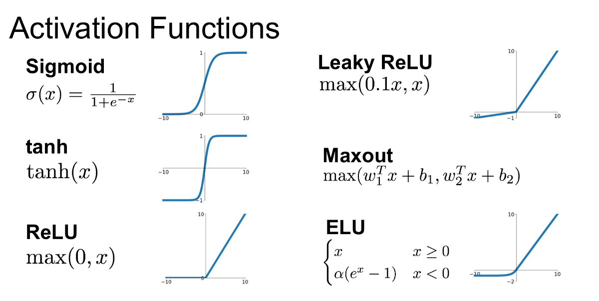Figure 1: Some of the more common activation functions (Jadon, 2019)

Testing and Configuration

After running a few evaluations of Team B’s dataset, we decided that because a lot of the sonic energy of these impact sounds was in the high end, it would improve the model to choose a sampling rate of 44.1kHz, which was the actual sample rate for our audio samples. During our feature selection, we found it difficult to discern which features dramatically improved the predictions as we weren’t able to simply A/B test the model. However, we did note that a large amount of features lead to the detriment of the model’s predictive ability. A fewer number of features were able to provide higher accuracy in our tests. This is likely due to too many irrelevant sonic features “polluting” the extraction of salient features within the sample pool. In an attempt to A/B test all of the features, we found that the only scalar feature that did not improve the model was spectral flatness. After testing several different activation functions and hidden layer counts and sizes, our best results ended up merely being a single layer with 100 nodes using the ReLU activation function.

Results?

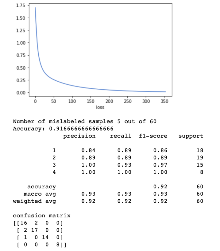Figure 2: Jarle’s results for one attempt

Building a model to categorize Team B’s dataset was largely successful, with an accuracy of 94% over a 10-fold validation (at our best, see Figure 3). Afterwards, we trained the model with another group’s dataset to compare whether our configuration would apply to another database: it did not. We found that Team B and Team C compiled very different datasets, resulting in less accurate classifiers built from the sample database. We were only able to achieve a consistent 70%, regardless it seemed, of changes to the activation function or hidden layer architecture. Team C’s sounds, it seemed from examination by ear, shared less sonic similarities, and appeared to be sourced from multiple different sample packs (shame on them!).

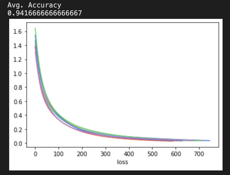Figure 3: Jackson’s results averaged over 10 iterations

In any case, through this module, we were able to learn quite a bit about the theory (and some practice) of basic machine learning. We trained an instrument using a readily made neural model to produce control dynamic synth in space and a classifier that was able to recognize categories of sound using their spectral qualities accurately. With this perspective, we did succeed in dipping our toes into the great big world of machine learning.

References

Fiebrink, Rebecca, and Perry Cook. “The Wekinator: A System for Real-Time, Interactive Machine Learning in Music.” Proceedings of The Eleventh International Society for Music Information Retrieval Conference (ISMIR 2010), Jan. 2010.

Jadon, Shruti. “Introduction to Different Activation Functions for Deep Learning.” Medium, 6 Nov. 2019, https://medium.com/@shrutijadon10104776/survey-on-activation-functions-for-deep-learning-9689331ba092.

Scikit-Learn: Machine Learning in Python — Scikit-Learn 0.21.3 Documentation. https://scikit-learn.org/stable/index.html. Accessed 23 Nov. 2019.

Quick Walkthrough of Wekinator. YouTube, https://www.youtube.com/watch?v=dPV-gCqy9j4. Accessed 25 Nov. 2019.