Machine Learning, it's all about the data
For my machine learning project, I wanted to see if I could teach my laptop to distinguish between different types of music using a large amount of data. Using metadata from a large dataset for music analysis, I tested different machine learning classifiers with supervised learning to distinguish between tracks labeled belonging to ‘Rock’ and ‘Electronic’. The project was developed using Python and libraries for data analysis and machine learning. I managed to make some progress in the end, but these things take time, so it is merely a preliminary dip into what machine learning can accomplish.
The dataset
Sourcing or collecting data can be both costly and time consuming, but luckily for me and others looking for large amounts of music data, someone has already done the work for us. I was lucky enough to find a dataset that was both large and applicable for the task at hand. FMA: A Dataset for Music Analysis is a large dataset containing free and legal music along with metadata and extracted features. The dataset is sourced from The Free Music Archive, and contains 917 GiB and 343 days of Creative Commons-licensed audio from 106,574 tracks from 16,341 artists and 14,854 albums. In other words, a whole lot of ones and zeroes.
Processing the audio in such a huge dataset would require too much time, so I would have to make do with the preprocessed metadata designating the different features and values for each track. The audio features for each track had been extracted using Librosa in Python, resulting in 518 values per track containing information and different statistics for the various features Librosa can extract. In the end, a file containing a list of all the tracks, their title, artist, and most importantly genre, was used together with a file containing all the audio features for each track. This still meant that I had 106,574*518 datapoints that needed to be organised before using it for machine learning.
Selecting columns and rows
Much like in an excel table, the data I was working with was organised in a .csv file, which Pandas, a data analysis toolkit for Python, can store and manipulate in many various ways. By selecting items with the genres I was looking for and picking the relevant columns, I made a new list of items that could be correlated with the features for each item. This selection numbered 18845 examples which were split with a 70/30 ratio for learning and testing. The last part was to select features and normalise the values.
Teaching the models
I tested four different machine learning algorithms with Scikit-learn to see how they performed both in accuracy and time. Each model gave an accuracy of its predictions, and using a Jupyter Notebook command I could see how long it took for the CPU to execute a given command.
Gaussian naïve bayes gave the worst result of the four models with an accuracy of about 66%, but it only took 24.9 ms to train the model.
K-nearest neighbour was also quick, but it performed much better with an accuracy of about 74%.
The Support Vector Machine I tried was much slower to train than the other models, using about 5.44 seconds. It also performed slightly lower than some of the others with about 72% accuracy.
The last model I tried was a Multilayer Perceptron, which is a basic neural network. This managed to get the best performance with 75% accuracy after tweaking some of the settings, ending up with four hidden layers of six neurons each. It was however also slower to train, taking 3.77 seconds.
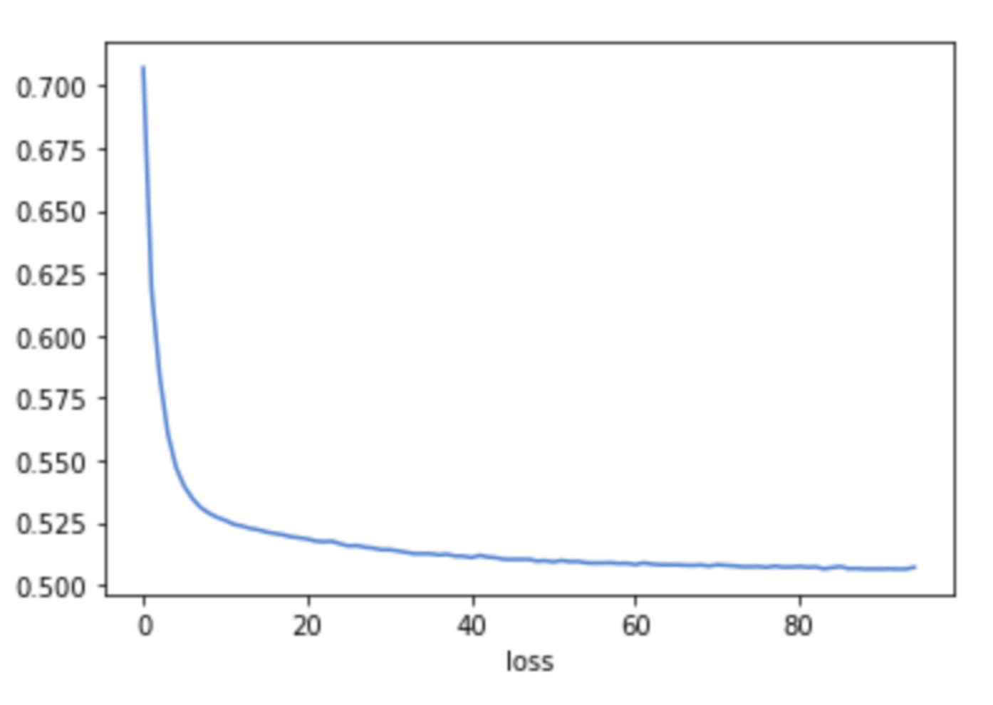
Below is a graph of the loss curve showing how the model improved its performance as it learns from the data.
Results
Was it really successful? Probably not. However, the results raise a few questions regarding the dataset, relevant features for genres, and techniques for separating classes better using dimensionality reduction. It’s all really about how the data is understood and presented for the machine which determines how well it’s going to perform.