Don't stop the music please, but please do

Introduction

This blog post will describe the process of taking two audio files and writing a Python program to slice and join the segments from both audio files based on the spectral centroid mean.

“Don’t stop the music” was first recorded and released in 2007 by Rihanna. The song was written by Tawanna Dabney and Norwegian production team StarGate. Jamie Cullum recorded a cover of the song in 2009, and it is these two versions that our team decided to chop up and put together based on features of the audio.

To combine these files, we started by using librosa to separate the harmonic and percussive content of the songs. This allowed us to more accurately use onset detection on our audio files using the percussive tracks, which then let us slice up into segments based on the onsets. The harmonic versions of the segments were used to find the spectral centroid of each segment, and we then each segment for both songs in ascending order based on the average value of the spectral centroid.

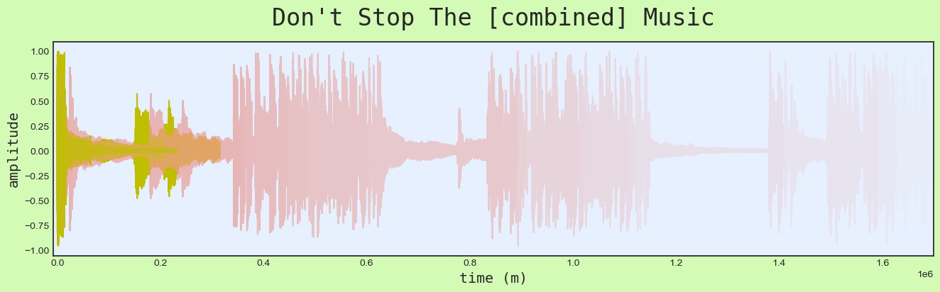
In the end we added the segments together one by one based upon spectral centroid average, creating a new audio file with all the segments from the two original tracks, but rejoined in a completely new way. You can view a block diagram of our process below.

Block diagram of our process

In our design, we decided to create a class for each song and stored a list of segment classes, which includes the audio array and the spectral centroid average value, in each song class. After creating a class for each segment, we sorted each segment based on the spectral centroid average value in a combined Pandas DataFrame, then used the indexes in the DataFrame to extract the correct audio segment from the class array.

Results

The two songs chosen for our re-synthesis:

Rihanna - Don’t Stop The Music

Jamie Cullum - Don’t Stop The Music (Cover)

By using two songs that are not really that similar but have the same foundation, we get some interesting artefacts in the re-synthesised audio. Since Rihanna’ original song is a dance-song, it emphasises the quarter notes. Cullum’s version uses sub-divisions to carry the song. This leads to the snare-drum from Cullum’s song appearing in some interesting places.

Since the re-synthesized song is arranged in ascending order based on the spectral centroid, it leads to sounding a bit musical and rhythmic. It sounds like a duet between Rihanna and Cullum, fighting each other for the spotlight. The duet-fight ends with Rihanna naturally winning the battle by bringing a dance song to the fight.

A thirteen seconds audio sample of our combined audio, taken in the middle of the full audio where there is more of a balance between Rihanna and Cullum’s contributions.

Challenges

Here you can see how each new segment also consists of the previous one(s). Rihanna's first segments shown in red, with opacity set to 5%. (Cullums segments in gush green are still on top of each other.)

We had an idea to plot the final audio as a traditional waveform, but with each segment color-coded to show it’s origin. This happened to be a much more complex task than anticipated. In the lack of managing to offset the coordinates along the X-axis so each new segment started where the previous left off, we approached it by filling in lots of zeros to offset them instead. Those zeros seemed so innocent, but oh my, how they teamed up against the CPU. It would often result in the code crashing. We later figured out that even if we could find a way to process and plot it all, which seemed close in sight several times, it would take too much time in the end.

5 subplots with 100 segments each. The timer above shows that it processed each subplot in good time. But below the plot you can see it took a lot of time to actually show the final plot.

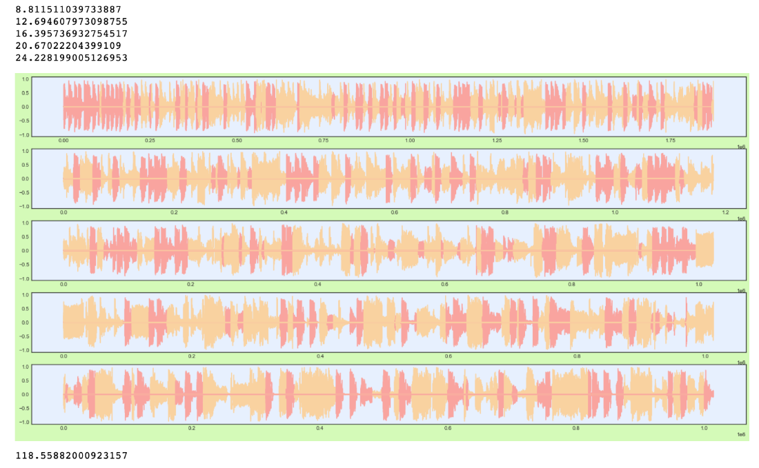
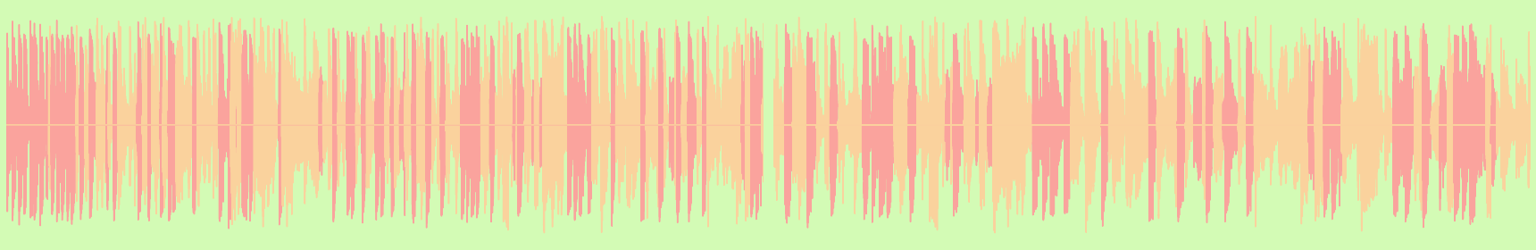
We tried different approaches. They were all based on using subplots with parts of the whole, to “reset” the ever-ascending pile of zeros lurking behind the scenes. In the figure above you can see how displaying 500 segments was doable, but this was almost as far as we could go without the code crashing. There were 987 segments in total, and we managed to plot 600 of them in about 3:30 minutes. We actually got confirmation – by printing a message for every 100 segments – that we were able to process them all. But there was no way it would show us the plot in the end. It took about 4:00 minutes to process, and small artifacts started to appear across the screen showing the struggle. Another approach was to make the subplots aligned horizontally without an axis and as close to each other as possible (with just a slight gap). This was the aesthetically most pleasing approach, and ended up being the way we visualized it in our code. Though for our final version, we thought it looked best with a “zoomed in” plot of only 100 segments. We found that different approaches had slight variations in time spent, but they all faced the same limits in the end. The process of finding a solution to make it work taught us a valuable lesson regarding CPU and time-consumption, and it forced us to think more cost-efficient overall.

2 subplots of 100 segments each, with their axis removed. You can see a slight gap between the subplots. We thought this approach was the most aesthetically appealing.

The source code for this assignment can be viewed here. To use this program for different sound files, you must first place two new wav files in a folder called “Files” in the same directory as the code. Once this is done, change the strings “song1” and “song2” to accurately reflect the files you want to process.